Does table size drive pot size? A LINER-checked walk through three tests on 1238 hands

Different table sizes produce visibly different hands at the same stake. Heads-up play grinds out in tight reraised pots; six-max tables see more limps than fireworks; full nine-handed games carry several callers all the way to the river. The natural conjecture is straightforward: more seated players generates more action, and more action accumulates more chips in the pot.

This post asks the question precisely. Does pot size grow linearly with the number of seated players? The dataset is 1238 captured hands from one site (Replay Poker) at one stake (1/2 NL Hold'em). The pedagogical structure follows the standard AP-Statistics inference procedure: for every candidate test, the conditions are checked first (LINER for regression, the chi-square three-condition list for contingency tables, the F-test conditions for nested model comparison), and the test is run only if the conditions hold. We begin with the most ambitious test — linear regression on raw pot size — find that several of its conditions fail badly, and do not run it. We then step down to a less demanding test (chi-square, which asks only whether there is any association at all), check its conditions, and run it. We then restore regression machinery on a scale where its conditions are defensible (log-linear), check, and run. Finally we ask whether the linear shape on the log scale is itself the right one, with a lack-of-fit F-test.

The goal is not to land on a clever single number. The goal is to show where each line of the standard inference output comes from, in arithmetic, and where the procedure tells us to stop before producing a number.

A reader's tour of the data

The exposition assumes familiarity with the rules of Texas Hold'em — blinds, hole cards, the four streets (preflop, flop, turn, river), and the actions bet, call, raise, fold, check, all-in. Statistical terminology is defined as it appears.

The dataset

Hands played on Replay Poker by users of the companion Chrome extension are uploaded to this site, where each hand becomes one row in a structured database. The /data page replays them individually; the /data/export-csv endpoint bundles a slice of the table into three CSV files: hands.csv, actions.csv, players.csv.

This post uses a single export of 1238 hands, all played at the same stake (1/2 NL Hold'em — small blind 1 chip, big blind 2 chips), spread across 6 distinct tables on the site. Joining the three CSVs yields one row per hand with all the information needed below.

The two columns of interest

• num_seats — the number of active players at the start of the hand. "Active" means the site reported them as occupying a seat with a stack when the hand was dealt; empty felt slots are filtered out by the export, so num_seats = 6 denotes six players actually receiving cards. This is the predictor variable $X$, ranging from $2$ to $9$.
• pot_BB — for each hand, the sum of every chip moved seat-to-pot through a voluntary action (bet, call, raise, allIn), divided by the big blind (= 2 chips). The mandatory blinds are excluded on purpose: they contribute a constant 1.5 BB floor in every hand regardless of seat count, which would shift the intercept of any model upward without affecting the slope. The metric is "voluntary chip volume per round, expressed in big blinds". This is the response variable $Y$.

A worked example: hand 1385727190 from the dataset, six seats, dealer at seat 5.

Street	Action	Voluntary chips this street
Preflop	Seat 5 raises to 4. Seats 0, 1, 2, 3, 4 call.	4·4 + 3 + 2 = 21 chips
Flop (Tc 7s As)	Seat 1 bets 24. Seat 2 folds; seats 3, 4, 5, 0 call.	24·5 = 120 chips
Turn (Ts)	Bet 2, four calls, seat 0 raises to 4, seat 1 raises to 6, calls and a clean-up call, seat 5 folds.	26 chips
River (Kc)	Everyone checks.	0 chips
Showdown	Cards revealed, pot awarded.	—

Voluntary total: $21+120+26+0=167$ chips $=83.5$ BB. The final pot at showdown included the 1.5 BB of blinds on top (giving 85 BB), but the pot_BB value recorded for this hand is 83.5. That is one row out of 1238.

Summary statistics

The empirical distribution of $X$ across seat counts:

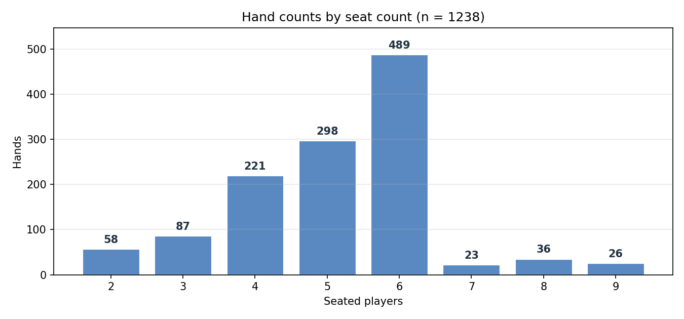
The bulk of the data lies at 4–6 seats. There are very few hands at 7–9 seats, and the majority of those come from a single full-ring table.

Pot sizes in BB are heavy-right-tailed:

Quantile	5 %	25 %	50 %	75 %	95 %
Pot (BB)	1.5	7.5	31.8	222.4	875.6

The sample mean is $\bar{y}=187.61$ BB but the median is only $31.8$ BB. The mean is roughly six times the median — the signature of a heavy right tail driven by a small number of very large all-in pots.

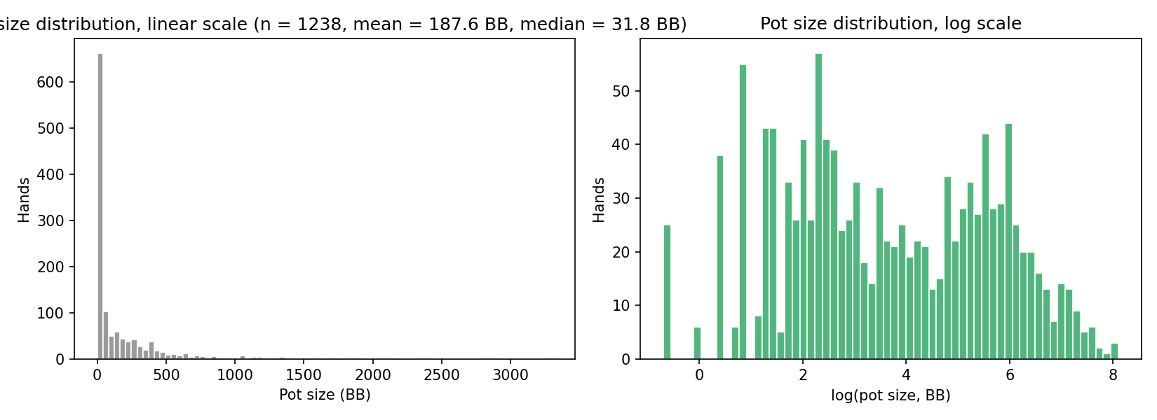
The left panel shows the raw histogram (one tall bar near zero plus a long sparse tail); the right panel shows the log-pot histogram, which is much more symmetric. The latter motivates the log transform used from Test B onward.

Six tables, six personalities

The 1238 hands originate from six different tables. They are not interchangeable:

Table	Hands	Seat range	Median pot (BB)	Mean pot (BB)
Duck Pond	349	2 – 6	22.5	195.6
Duck Pond 2	218	2 – 6	12.2	49.6
Duck Pond 3	138	2 – 6	217.0	393.4
Duck Pond 5	166	3 – 6	47.5	153.5
Duck Pond 6	202	2 – 6	14.5	109.8
Aquarium	165	3 – 9	163.0	310.4

The median pot is roughly 18× larger at Duck Pond 3 (217 BB) than at Duck Pond 2 (12.2 BB). Both tables share the same modal seat count, so this gap is not driven by seat count; it reflects who is seated and how they play. Aquarium is the only table that ran 7–9-handed during the capture window, so almost all 7–9-seat data points originate from one table.

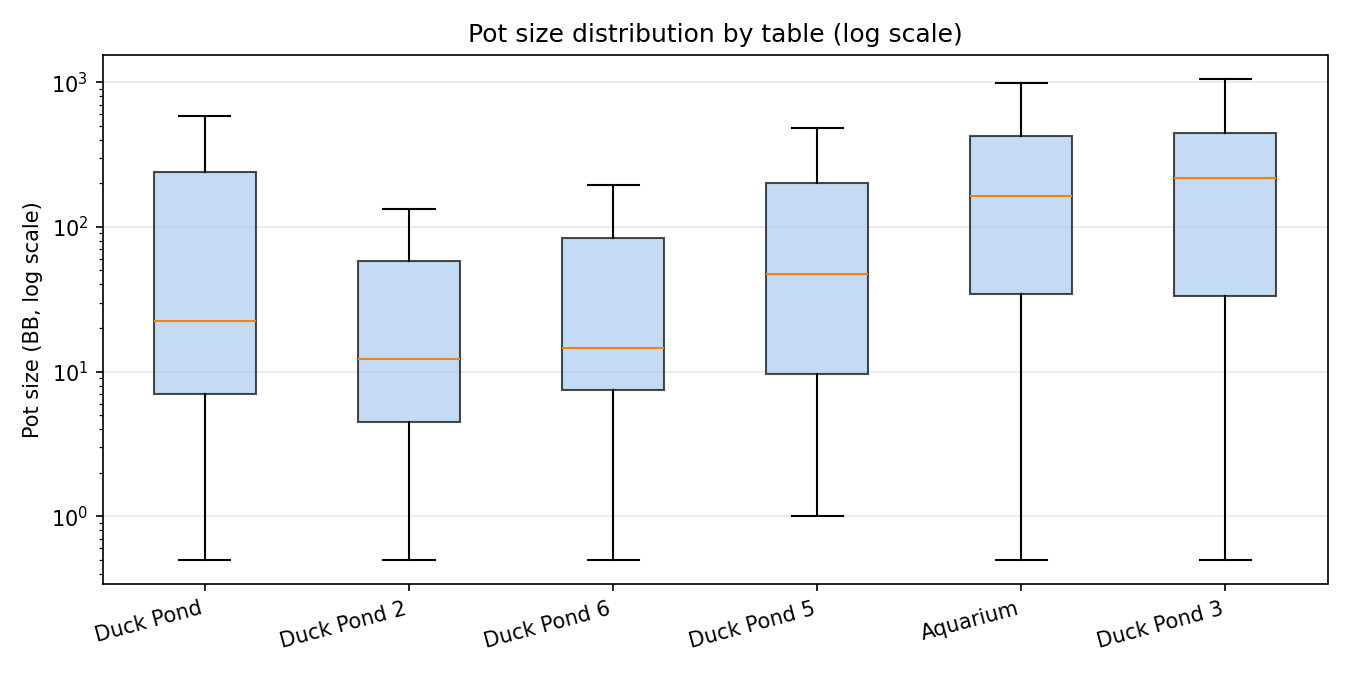
This picture matters when the independence condition is examined below: it is the visual evidence that the table itself induces a shared component in the pot size of every hand played there.

The hypothesis

The substantive hypothesis is: more seated players produces (on average) bigger pots, in a straight-line relationship. Translated into a regression model with $i$ indexing hands:

$${\text{pot\_BB}}_i={\beta }_0+{\beta }_1\cdot {\text{num\_seats}}_i+{\epsilon }_i$$

Here ${\beta }_0$ is the intercept (the predicted pot at zero seats — not physically meaningful but mathematically required), ${\beta }_1$ is the slope in BB per added seat, and ${\epsilon }_i$ is the residual: whatever the line fails to capture on hand $i$. The null hypothesis is $H_0:{\beta }_1=0$ (seat count has no effect on pot size); the alternative is $H_A:{\beta }_1\ne 0$.

The natural test for this hypothesis is the regression slope t-test, which is valid under the LINER conditions:

• Linearity — the true relationship is a straight line.
• Independence — the $n$ observations are independent draws.
• Normality — the residuals are approximately bell-shaped.
• Equal variance — residuals have the same spread at every $X$.
• Random — the data form a random sample (or come from a randomized experiment).

When LINER holds, the slope t-test produces honest standard errors, t-statistics, p-values, and confidence intervals. When LINER fails, the test still produces numbers — but those numbers are no longer trustworthy. The conditions are checked below.

The post structure follows directly from these checks. Once raw-scale regression fails its conditions, the analysis steps down to two more modest questions and only runs what its conditions allow:

• Test A — Chi-square test of independence. The loosest question available: is there any association between seat count and pot size, of any shape? Distribution-free for $Y$.
• Test B — Log-linear regression slope t-test. Once association is established, this estimates the slope on the $\log (\text{pot})$ scale, where the regression conditions are defensible.
• Test C — Lack-of-fit F-test on the log scale. Once a linear-on-log slope is in hand, this tests whether the linear shape itself is appropriate, or whether the data require something more flexible.

A shared concern: independence

One condition argument applies to all three tests run below, so it is stated once here and referenced later as the I of LINER (and as the second condition of the chi-square test).

The case for independence. Each Replay Poker hand is dealt from a freshly shuffled virtual deck. The cards in hand 48 carry no information about the cards in hand 47 — there is no shared deck, no carryover, no mechanism by which one hand's randomness leaks into the next. The structural source of randomness in pot_BB (the dealt cards) is genuinely independent across hands.

The case for caution. Pot size is shaped by behavior on top of cards, and behavior at the same table over the same session can be correlated. Fifty hands played over an hour at "Duck Pond 6" share the same six players, the same blind level, possibly the same active maniac, possibly the same shared mood. If a player has just stacked off and is on tilt, hand 48 may inherit some of that tilt from hand 47. Across tables, table personalities differ — Duck Pond 3's median pot is roughly $18\times$ larger than Duck Pond 2's despite similar modal seat counts (visible in the by-table boxplot above).

Independence therefore holds cleanly at the level of cards but imperfectly at the level of player mentality.

Verdict: pass, with a warning. The dealt-cards argument captures the dominant source of variance in pot size; without that randomness, pot size would be deterministic given seat composition, which it clearly is not. The behavioral correlations are real but second-order on the variance budget, and the standard inference procedure treats such observations as effectively independent. The analysis proceeds as if the 1238 hands are iid, with the explicit warning that within-table dynamics may inflate test statistics by a small amount; the conclusions below should be read as "robust under iid plus a modest correction".

This argument is the same for every test below — each I check below references "pass, with the warning above". The other LINER conditions are test-specific, and they are checked immediately before each test in the way the inference procedure prescribes.

Why a raw-scale OLS slope t-test is not run

The default analytic move would be: fit $\text{pot\_BB}={\beta }_0+{\beta }_1\cdot \text{num\_seats}+\epsilon$ by least squares, compute $t={\hat{\beta }}_1/\mathrm{SE}({\hat{\beta }}_1)$, and report a p-value. The procedure prescribes a LINER check before that p-value is reported; if LINER fails, the t-statistic and the resulting p-value are not trustworthy. The check follows below.

LINER check on raw OLS

L — Linearity. The cleanest diagnostic is to scatter every hand on $(\text{seats},\text{pot})$ with linear axes, plot the bin means at each seat count, and overlay the would-be OLS line:

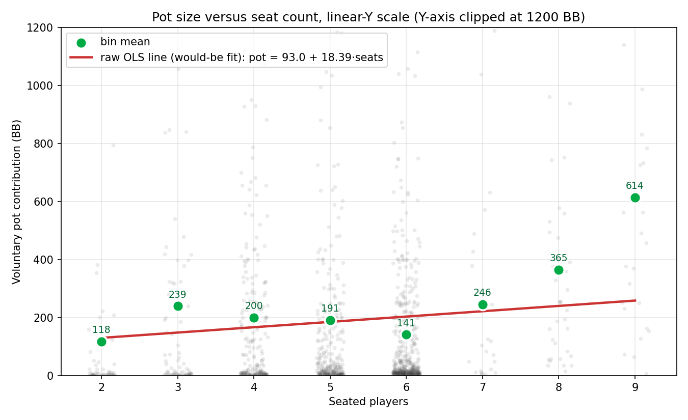
The bin means (green) rise from 118 BB at 2 seats to 239 BB at 3 seats, fall through $200\to 191\to 141$ BB across 4–5–6 seats, then explode to $246\to 365\to 614$ BB at 7–8–9 seats. The trajectory is non-monotonic — up, down, then up again. The OLS line (red) cuts straight through, missing every bin mean by 50–350 BB. (The y-axis is clipped at 1200 BB so the structure is visible; a few outlier hands had pots of several thousand BB and fall outside the panel.)

A straight line is the wrong shape for this cloud. Verdict: L fails.

I — Independence. Pass, with the warning discussed above. The cards are dealt from a fresh shuffle every hand, so the structural randomness is independent; only the behavioral component carries weak within-table correlations.

N — Normal residuals. The $Y$ distribution is heavily right-skewed (mean 188 BB, median 32 BB, 95th percentile 876 BB; see the left panel of the histogram above). The residuals from a linear fit inherit that skew almost completely — fitted values lie between 130 and 260 BB, but actual pots range from 1.5 to several thousand BB. A histogram of residuals would show one tall spike near zero and a long right tail. Verdict: N fails dramatically.

E — Equal variance. Within each seat-count bin, the spread of pot sizes varies enormously. At 2 seats, most pots are tiny (median 5.5, 75th percentile around 30). At 9 seats, most pots are large (median 474, 75th percentile much larger). The within-bin standard deviation grows by an order of magnitude from 2 seats to 9 seats. Verdict: E fails.

R — Random sample. Pass — and the reasoning is worth stating explicitly, because random sampling is the one LINER condition where this dataset is better than most observational data.

Two upload paths feed the database, and both are randomized by protocol:

1. Generic uploads come exclusively from the site administrator. The choice of which tables and sessions to capture is randomized; the administrator deliberately does not cherry-pick interesting hands or focus on any one table. The crawler effectively samples uniformly across the table catalog, with no relationship between which hands get uploaded and the pot size that results.
2. Per-user uploads come from individual extension users, who are instructed in the user guide to upload sessions chosen at random rather than memorable hands. Because pot size is decided after the upload selection, there is no mechanism for the selection to bias the outcome variable.

Both paths sample without reference to the value of pot_BB, so the 1238 hands are exchangeable in the sense the random-sample condition requires. Verdict: R passes.

Decision

Of the five LINER conditions, three fail (L, N, E) and two pass (I with warning, R). The procedure for failing conditions is unambiguous: do not run the test. Even with I and R intact, the failures of L, N, and E are individually fatal — the OLS slope ${\hat{\beta }}_1$ exists as an arithmetic object (the formula is always defined), but the inference (the t-statistic, p-value, and confidence interval) is not justified, because the sampling distribution underlying it does not apply to data with this shape and this residual structure.

No p-value or CI from the raw-scale slope test is therefore reported. The only honest takeaway from the raw-scale picture is that the bin means are not even monotonic — which is itself evidence that the right question is a different one.

The path forward is three steps, in increasing precision:

1. Ask only "is there any relationship between seats and pot, of any shape?" — a question that does not require LINER to hold. This is what the chi-square test of independence does.
2. Once association is established, restore regression machinery on a transformed scale where the regression conditions are defensible — the log-linear test.
3. On that transformed scale, ask whether linearity is itself the right shape, via a lack-of-fit F-test.

All three are run, in order, below.

Test A — Chi-square test of independence

Purpose. Before asking "what is the slope?" or "what is the shape?", the analysis should first establish that there is anything worth measuring. The chi-square test of independence is the loosest tool available for this question: it bins both variables into categories and asks whether the resulting contingency table looks more uneven than chance allows. It does not commit to a slope, a sign, a shape, or a distribution for $Y$. The price for that freedom is information loss from binning.

Conditions for the chi-square test

The chi-square test of independence carries three standard conditions:

(1) Random — observations form a random sample. Pass, by the same upload-protocol argument as in the regression LINER check above. The 1238 hands are sampled without reference to their pot size, both for administrator-driven generic uploads and for per-user uploads.

(2) Independence — the observations are independent of each other. Pass, with the warning documented above. Each hand's cards are dealt independently of every other hand's cards; behavioral correlations within a table session are real but second-order.

(3) Large enough expected counts — every cell's expected count must satisfy $E_{ij}\ge 5$ (the standard rule of thumb). This condition depends on the binning, so it must be evaluated after the expected counts are computed. As shown in the arithmetic below, the smallest expected count is 20.32, comfortably above 5. Pass.

This test does not require normality, equal variance, or a linear shape — those are regression conditions. The heavy right tail of pot sizes that killed raw-scale OLS does not threaten the chi-square test.

Decision: proceed, with the iid disclaimer attached to the resulting p-value.

Algorithm

For an $r\times c$ contingency table with cell counts $O_{ij}$:

1. Compute row totals $R_i={\sum }_j{O}_{ij}$, column totals $C_j={\sum }_i{O}_{ij}$, and grand total $N={\sum }_{ij}{O}_{ij}$.
2. Compute the expected count in each cell under the null hypothesis that $X$ and $Y$ are independent:

$$E_{ij}=\frac{R_i\cdot C_j}{N}$$

3. The test statistic is

$${\chi }^2=\sum _{i,j}\frac{(O_{ij}-E_{ij}{)}^2}{E_{ij}}$$

4. Under $H_0$ and the condition $E_{ij}\ge 5$ in every cell, ${\chi }^2$ follows a chi-square distribution with $\mathrm{df}=(r-1)(c-1)$.
5. Cramer's V measures effect size on a $[0,1]$ scale (small $\le 0.1$, medium $\approx 0.3$, large $\ge 0.5$):

$$V=\sqrt{\frac{{\chi }^2}{N\cdot (\min (r,c)-1)}}$$

Choosing the bins

Binning is a methodological choice. The bins used are:

• Seat-count tiers (4 levels): HU/3-max (2–3 seats), 4–5, 6-max (just 6), full ring (7–9).
• Pot quartiles (4 levels): tiny ($\le 7.5$ BB), small ($7.5$–$31.8$), medium ($31.8$–$222.4$), big ($>222.4$). Quartiles guarantee equal-sized columns (309 or 310 hands each), which keeps the expected counts comfortably above 5 even in the smallest row.

Plugging the numbers in

Observed counts $O_{ij}$ (rows are seat tiers, columns are pot quartiles):

seats \ pot	tiny	small	medium	big	$R_i$
HU / 3-max	66	24	24	31	145
4–5 seats	138	109	140	132	519
6-max	115	157	118	99	489
Full ring (7–9)	4	6	27	48	85
$C_j$	323	296	309	310	$N=1238$

The expected counts are $E_{ij}=R_i\cdot C_j/N$. The first row of the expected table, computed explicitly:

$$\begin{array}{rl}E(\text{HU},\text{tiny})& =\frac{145\cdot 323}{1238}=\frac{46,835}{1238}=37.83\\ E(\text{HU},\text{small})& =\frac{145\cdot 296}{1238}=\frac{42,920}{1238}=34.67\\ E(\text{HU},\text{medium})& =\frac{145\cdot 309}{1238}=\frac{44,805}{1238}=36.19\\ E(\text{HU},\text{big})& =\frac{145\cdot 310}{1238}=\frac{44,950}{1238}=36.31\end{array}$$

Sanity check: $37.83+34.67+36.19+36.31=145.00$, matching the row total.

Repeating for every row gives the full expected table. The per-cell contributions $(O_{ij}-E_{ij}{)}^2/E_{ij}$ follow by element-wise arithmetic. The figure below shows the three matrices side-by-side as heatmaps:

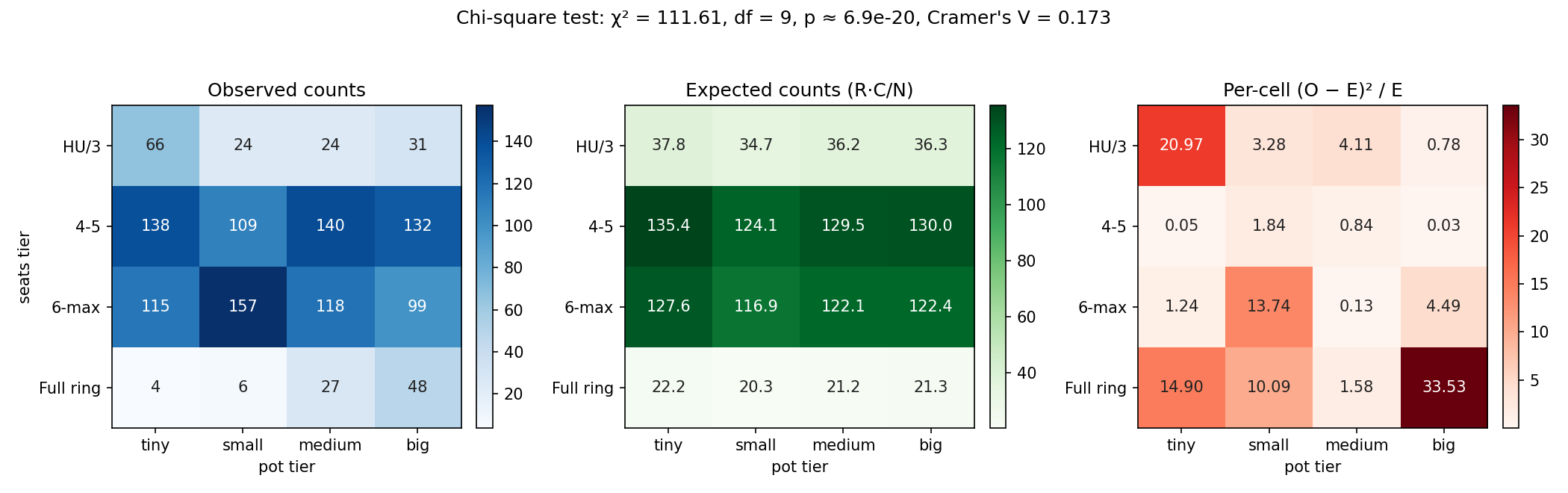
The leftmost panel shows the observed counts (the same numbers as the table above, colored). The middle panel shows the expected counts under $H_0$. The rightmost panel shows the per-cell contribution to ${\chi }^2$. The bottom-right cell (full ring $\times$ big pot) contributes 33.55 to ${\chi }^2$ on its own:

$$\frac{(48-21.28{)}^2}{21.28}=\frac{26.72^2}{21.28}=\frac{713.96}{21.28}=33.55$$

The smallest expected count anywhere is 20.32, well above the rule-of-thumb threshold of 5, so the chi-square approximation is valid.

Summing all sixteen cell contributions yields the test statistic:

$${\chi }^2=29.14+2.76+19.61+60.10=111.61$$

These four numbers are the row sums of the rightmost panel: HU/3-max contributes 29.14, the 4–5 row contributes only 2.76, 6-max contributes 19.61, and full ring contributes 60.10.

Two rows carry the bulk of the story. The 4–5 row contributes only 2.76 — observed counts there are close to expectation everywhere, so 4–5-seat hands are typical. The full-ring row contributes 60.10, more than half the total — full-ring hands are very different from expectation, with too few small pots and far too many big ones.

Degrees of freedom: $\mathrm{df}=(4-1)(4-1)=9$.

The p-value is the upper-tail probability of a ${\chi }_9^2$ random variable exceeding 111.61:

$$p=\mathrm{Pr}({\chi }_9^2>111.61)\approx 6.9\times 10^{-20}$$

For comparison, the $\alpha =0.001$ critical value of ${\chi }_9^2$ is 27.88 — the observed statistic of 111.61 is roughly four times larger, which is why the p-value is microscopic.

The effect size:

$$V=\sqrt{\frac{111.61}{1238\cdot 3}}=\sqrt{\frac{111.61}{3714}}=\sqrt{0.03005}=0.173$$

Reading the result

• $p\approx 6.9\times 10^{-20}$ rejects $H_0$ ("seat tier and pot tier are independent") at any sane significance level. There is a relationship between table size and pot size.
• Cramer's V $=0.173$ is in the small-effect range. The relationship is overwhelmingly real, but it does not predict the pot size of a single hand from its seat count with much accuracy; it only shifts the probability distribution of pot tiers in a measurable direction.
• The location of the effect is identified by the cell contributions: full-ring hands skew strongly toward big pots, HU/3-max hands skew toward tiny pots, and the middle two tiers track expectation closely. This hints at a non-linear relationship concentrated in the extremes.
• What this test does not deliver: any slope, sign, or directed-magnitude statement. It only asserts the existence of some dependence between two ordered categorical variables.

Test B — Log-linear regression

Purpose. Test A confirmed that some relationship exists. The obvious next question is how large the relationship is, expressed as a single number. The natural such number is the slope of a regression line. A slope test on raw pot_BB is unavailable because LINER failed on that scale. The standard remedy when residuals are right-skewed and heteroscedastic is to model $\log (\text{pot\_BB})$ instead, and then apply the same regression machinery on the new scale where its conditions may actually hold.

The model becomes

$$\log ({\text{pot\_BB}}_i)={\beta }_0+{\beta }_1\cdot {\text{num\_seats}}_i+{\epsilon }_i,$$

which is algebraically equivalent to

$${\text{pot\_BB}}_i=e^{{\beta }_0}\cdot (e^{{\beta }_1}{)}^{{\text{num\_seats}}_i}\cdot e^{{\epsilon }_i}.$$

The slope ${\beta }_1$ is no longer "BB added per seat"; it is the natural log of the multiplicative factor by which the typical pot grows per seat. For example, ${\hat{\beta }}_1=0.10$ corresponds to each extra seat multiplying the typical pot by $e^{0.10}\approx 1.105$ — a 10.5 % increase per seat.

LINER check on log-linear regression

The same five conditions are evaluated on the new model ($\log (\text{pot})$ as response, $\text{num\_seats}$ as predictor):

L — Linearity. Genuinely uncertain. A line on the log scale corresponds to an exponential on the raw scale, which is a stronger restriction than "any monotonic shape". The analysis tentatively assumes linearity here, runs the slope test, and tests the linearity assumption directly with the lack-of-fit F (Test C). Verdict for now: assumed; checked rigorously in Test C.

I — Independence. Pass, with the warning above. The dealt-cards argument applies on the log scale just as on the raw scale; behavioral correlations remain a second-order concern.

N — Normal residuals. The right panel of the histogram figure shows the distribution of $\log (\text{pot\_BB})$. It is roughly bell-shaped, slightly left-skewed, with no extreme tail. The residuals from a regression on this response inherit essentially the same shape after a small constant trend is removed, so they will also be approximately bell-shaped. Verdict: pass.

E — Equal variance. The standard diagnostic is to compute the within-bin standard deviation of the response at each $X$ and check that the spreads are similar:

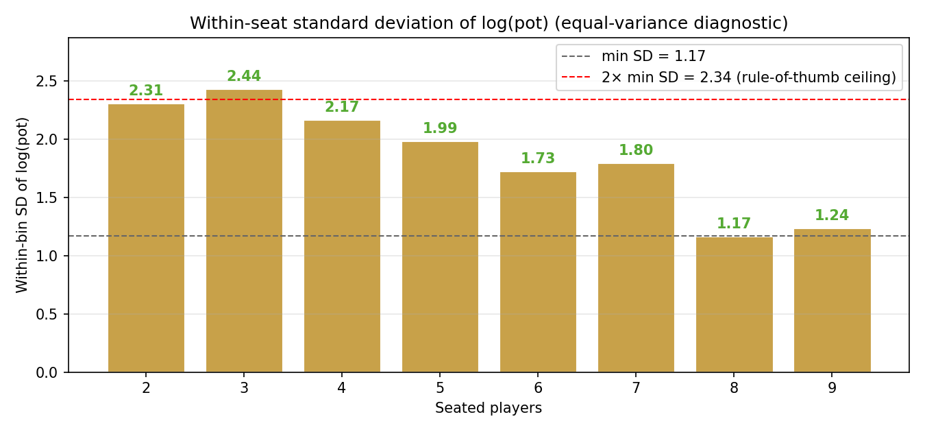
The within-bin SDs range from 1.17 (at 8 seats) to 2.44 (at 3 seats) — a ratio of roughly $2.09$. The standard rule of thumb is "largest SD $\le 2\times$ smallest"; the observed ratio just clears that ceiling. The small-$n$ bins at 8 and 9 seats (36 and 26 hands) produce noisy SD estimates, so the visible spread there should be discounted somewhat. The dashed red line marks the $2\times$ ceiling and most bars sit comfortably below it. Verdict: marginal-pass.

For contrast, on the raw-$Y$ scale the within-bin SD grows by an order of magnitude across bins. The log transform is doing real work here.

R — Random sample. Same justification as the raw-OLS check above — the upload protocol is randomized at both the administrator level and the per-user level, so the 1238 hands form a random sample from the population of hands the extension is configured to capture. Verdict: pass.

Decision: of the five LINER conditions, four pass (I with warning, N, E with marginal pass, R) and one is assumed for now and tested in Test C (L). The combination is enough to proceed, with a Test C follow-up scheduled.

Algorithm

The same OLS slope-test machinery that would have been used for raw OLS, applied with ${\ell }_i=\log (y_i)$ substituted for $y_i$. The relevant centered sums are

$$S_{x\ell }=\sum _i(x_i-\bar{x})({\ell }_i-\bar{\ell }),S_{\ell \ell }=\sum _i({\ell }_i-\bar{\ell }{)}^2.$$

Then the standard formulas carry over:

$$\begin{array}{rl}{\hat{\beta }}_1^{(\log )}& =S_{x\ell }/S_{xx},\\ {\hat{\beta }}_0^{(\log )}& =\bar{\ell }-{\hat{\beta }}_1^{(\log )}\cdot \bar{x},\\ {\mathrm{SSE}}_{\log }& =S_{\ell \ell }-{\hat{\beta }}_1^{(\log )}\cdot S_{x\ell },\\ s_{\log }& =\sqrt{{\mathrm{SSE}}_{\log }/(n-2)},\\ \mathrm{SE}\left({\hat{\beta }}_1^{(\log )}\right)& =s_{\log }/\sqrt{S_{xx}},\\ t_{\log }& ={\hat{\beta }}_1^{(\log )}/\mathrm{SE}\left({\hat{\beta }}_1^{(\log )}\right)\text{with }\mathrm{df}=n-2.\end{array}$$

Plugging the numbers in

From the $1238$ pairs $(x_i,y_i)$, the $X$-related sums are:

$$\begin{array}{rl}n& =1238\\ \sum _i{x}_i& =6,368\\ \sum _i{x}_i^2& =35,142\\ \bar{x}& =6368/1238=5.14378\\ S_{xx}& =35,142-6368^2/1238=2,386.41\\ \mathrm{df}& =n-2=1236\\ t^{\ast }& =t_{0.975,1236}\approx 1.962\end{array}$$

The same critical value $t^{\ast }$ governs both the slope CI here and the lack-of-fit reference distribution in Test C; with $\mathrm{df}>1000$ the $t$-distribution is essentially normal.

The $Y$-related sums on the log scale:

$$\bar{\ell }=3.6097,S_{\ell \ell }=5,037.24,S_{x\ell }=\mathrm{699.13.}$$

Note that $e^{3.61}\approx 37$ BB. The geometric mean pot is about 37 BB, much closer to the median 32 BB than to the arithmetic mean 188 BB — precisely because the log transform pulls the heavy right tail in.

The slope and intercept on the log scale:

$${\hat{\beta }}_1^{(\log )}=\frac{699.13}{2386.41}=0.2930\text{(log-BB per seat)},{\hat{\beta }}_0^{(\log )}=3.6097-0.2930\cdot 5.144=\mathrm{2.1028.}$$

The fitted line is $\log (\text{pot\_BB})\approx 2.103+0.293\cdot \text{num\_seats}$, which exponentiates to $\text{pot\_BB}\approx e^{2.103}\cdot e^{0.293\cdot \text{seats}}=8.19\cdot 1.340^{\text{seats}}$. The model therefore predicts roughly $14.7$ BB at 2 seats ($=8.19\cdot 1.340^2$), $26.5$ BB at 4 seats, $47.5$ BB at 6 seats, and $85.4$ BB at 8 seats.

The same scatter on a log-Y axis, with the fit and 95 % CI band overlaid:

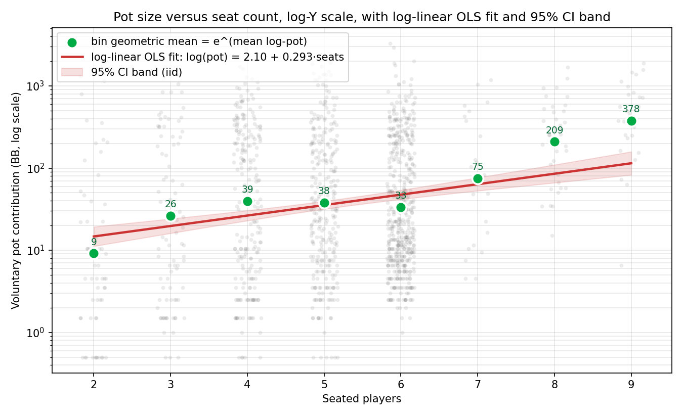
The green markers (bin geometric means) hug the red curve much more closely than the linear-Y bin means hugged the linear line back in the raw-OLS section. Systematic departures remain — the 8-seat and 9-seat geometric means sit clearly above the line — and these departures are precisely what Test C will detect.

The residual sum of squares and $R^2$:

$${\mathrm{SSE}}_{\log }=S_{\ell \ell }-{\hat{\beta }}_1^{(\log )}\cdot S_{x\ell }=5037.24-0.2930\cdot 699.13=4832.42,$$ $$R_{\log }^2=1-\frac{4832.42}{5037.24}=\mathrm{0.0407.}$$

The fit explains 4.07 % of the variation in log-pot. A straight line fits the data poorly in absolute terms, but this is still a meaningful improvement over the raw scale (where, if the test had been run, $R^2$ would have been about $0.5$ %).

The residual standard error:

$$s_{\log }^2=\frac{4832.42}{1236}=3.9097,s_{\log }=\sqrt{3.9097}=\mathrm{1.9773.}$$

A residual SE of 1.977 on the log scale means a typical hand's pot lands within a factor of $e^{1.977}\approx 7.2$ of the line's prediction. Substantial scatter, but in the expected range for poker variance.

The slope's standard error:

$$\mathrm{SE}\left({\hat{\beta }}_1^{(\log )}\right)=\frac{s_{\log }}{\sqrt{S_{xx}}}=\frac{1.9773}{48.851}=\mathrm{0.04048.}$$

Test statistic:

$$t_{\log }=\frac{{\hat{\beta }}_1^{(\log )}}{\mathrm{SE}\left({\hat{\beta }}_1^{(\log )}\right)}=\frac{0.2930}{0.04048}=\mathrm{7.238.}$$

A $t$-statistic of $7.24$ on $1236$ degrees of freedom is enormous. The two-sided p-value:

$$p_{\log }=2\cdot \mathrm{Pr}(T_{1236}>7.238)\approx 8.0\times 10^{-13}.$$

The 95 % CI on the log slope:

$${\hat{\beta }}_1^{(\log )}\pm t^{\ast }\cdot \mathrm{SE}\left({\hat{\beta }}_1^{(\log )}\right)=0.2930\pm 1.962\cdot 0.04048=0.2930\pm 0.0794=[0.2136,0.3724].$$

Exponentiating to recover the multiplicative interpretation:

$$e^{{\hat{\beta }}_1^{(\log )}}=e^{0.2930}=1.340\times \text{per seat},e^{4{\hat{\beta }}_1^{(\log )}}=e^{1.172}=3.23\times \text{(HU}\to \text{6-max)}.$$

The 95 % CI for the multiplicative effect is $[e^{0.214},e^{0.372}]=[1.238\times ,1.451\times ]$ per seat.

Reading the result

• $p_{\log }\approx 8\times 10^{-13}$ rejects $H_0:{\beta }_1^{(\log )}=0$ at any sane significance level. Under the LINER conditions just verified (with the iid disclaimer attached), there is overwhelming evidence that the typical pot grows with seat count.
• The point estimate: each extra seat multiplies the typical pot by $1.34$. Moving from heads-up (2 seats) to 6-max therefore multiplies the pot by $1.34^4\approx 3.23$. The 95 % CI for the multiplicative effect is $[1.238\times ,1.451\times ]$ per seat.
• $R^2=4.07$ %. A line on the log scale fits better than the same line on the raw scale would have, but it is still a thin description: 96 % of the variation in $\log (\text{pot})$ is unexplained. Most of that residual variance is irreducible "different hands play differently" noise that no model on seat count alone could capture.
• The large $t=7.24$ is largely a residual normalisation effect. On the raw scale, residuals of $\pm 300$ BB drown out the slope of $18.4$ BB per seat; on the log scale, residuals of $\pm 2$ log-BB make the slope of $0.293$ stand out clearly. Same data, much better signal-to-noise ratio.

Test C — Lack-of-fit F-test on the log scale

Purpose. Test B reported a slope on the log scale, but it had to assume linearity (the L of LINER). The lack-of-fit F-test now checks that assumption directly. The test compares the linear-on-log model to a more flexible saturated model that lets each num_seats value have its own log-mean. If the saturated model fits substantially better than the line, the data is signaling that "linear is wrong" — and Test B's slope was a lossy summary of something with more structure.

The test runs on the same log scale as Test B, because that is where the regression's other LINER conditions held. Running it on the raw scale would push back into the territory where N and E failed.

When $X$ has many repeats — as it does here, with $\text{num\_seats}\in \{2,3,\dots ,9\}$ and dozens to hundreds of hands at each value — a clean test for the linearity assumption is available.

Conditions for the lack-of-fit F-test

The F-test is a regression test and inherits LINER, with two specific differences from the slope t-test:

N — Normal residuals. Same as Test B's check, since the residuals are the same. Pass.

E — Equal variance. Same as Test B's check. The numerator of $F$ estimates "extra variability captured by the bins"; the denominator estimates "noise around the bin means". For both terms to be calibrated correctly, residual variance must be roughly constant across $X$. Marginal-pass on the log scale, as established.

I — Independence. Pass, with the warning above. The F-test would be anti-conservative under heavy clustering, but the dominant source of variance (dealt-card randomness) is genuinely independent.

R — Random sample. Pass, as established above.

L — Linearity. This is the hypothesis under test, so it is not pre-checked; $H_0$ for this test is "L is true".

Repeated $X$-values. Specific to the F-test (replaces L as the "must hold" condition): the test only works because of multiple observations at each of the 8 distinct seat counts. The smallest bin (7 seats) still contains 23 hands, plenty for a within-bin variance estimate. Pass.

Decision: proceed.

Algorithm

Fit two nested models on the log scale:

• Linear model (2 parameters): $\log (\text{pot\_BB})={\beta }_0+{\beta }_1\cdot \text{num\_seats}$. Residual SS is ${\mathrm{SSE}}_{\text{lin}}=4832.42$ (carried over from Test B). Residual df is $n-2=1236$.
• Saturated model (one parameter per distinct $X$ value): $\log (\text{pot\_BB})={\mu }_{\text{seats}}$. With 8 distinct seat counts this model has 8 parameters: it fits the mean log-pot at each seat count with no constraint on how those means relate. Residual SS is ${\mathrm{SSE}}_{\text{sat}}={\sum }_k{\sum }_{i\in \text{bin }k}({\ell }_i-{\bar{\ell }}_k{)}^2$ where ${\bar{\ell }}_k$ is the mean log-pot at seat count $k$. Residual df is $n-8=1230$.

The F statistic compares the two:

$$F=\frac{({\mathrm{SSE}}_{\text{lin}}-{\mathrm{SSE}}_{\text{sat}})/({\mathrm{df}}_{\text{lin}}-{\mathrm{df}}_{\text{sat}})}{{\mathrm{SSE}}_{\text{sat}}/{\mathrm{df}}_{\text{sat}}}.$$

Under $H_0$ (the linear-on-log model is adequate), $F$ follows an $F$ distribution with $({\mathrm{df}}_{\text{lin}}-{\mathrm{df}}_{\text{sat}},{\mathrm{df}}_{\text{sat}})=(6,1230)$ degrees of freedom. The numerator measures the extra variation the saturated model captures beyond the line, per added parameter. The denominator is the irreducible noise around the per-bin log-means.

Plugging the numbers in

${\mathrm{SSE}}_{\text{lin}}=4832.42$ is already in hand from Test B. To get ${\mathrm{SSE}}_{\text{sat}}$ the within-bin residual sums of squares on the log scale are needed. The per-bin log-means and counts:

seats	$n_k$	mean log-pot ${\bar{\ell }}_k$	within-bin SD of log-pot
2	58	2.213	2.31
3	87	3.269	2.44
4	221	3.676	2.17
5	298	3.633	1.99
6	489	3.507	1.73
7	23	4.313	1.80
8	36	5.343	1.17
9	26	5.935	1.24

The saturated SSE is the total within-bin variation:

$${\mathrm{SSE}}_{\text{sat}}=\sum _k\sum _{i\in \text{bin }k}({\ell }_i-{\bar{\ell }}_k{)}^2=\mathrm{4647.48.}$$

The differences:

$${\mathrm{df}}_{\text{lin}}-{\mathrm{df}}_{\text{sat}}=1236-1230=6,{\mathrm{SSE}}_{\text{lin}}-{\mathrm{SSE}}_{\text{sat}}=4832.42-4647.48=\mathrm{184.94.}$$

The numerator (mean square for lack of fit):

$${\mathrm{MS}}_{\text{LoF}}=\frac{184.94}{6}=\mathrm{30.82.}$$

The denominator (mean square for pure error):

$${\mathrm{MS}}_{\text{PE}}=\frac{4647.48}{1230}=\mathrm{3.778.}$$

The test statistic:

$$F=\frac{{\mathrm{MS}}_{\text{LoF}}}{{\mathrm{MS}}_{\text{PE}}}=\frac{30.82}{3.778}=\mathrm{8.158.}$$

Reference: $F$-distribution with $\mathrm{df}=(6,1230)$. The critical value at $\alpha =0.05$ is $F^{\ast }(6,1230)\approx 2.106$; the observed $F=8.158$ is roughly four times that. The exact p-value:

$$p=\mathrm{Pr}(F_{6,1230}>8.158)\approx 1.14\times 10^{-8}.$$

Reading the result

• $p\approx 10^{-8}$ rejects $H_0$ ("a line on the log scale is the right shape") at any significance level. Even after the log transform, the linear model is not the right model.
• Specifically: the line on the log scale has $\mathrm{SSE}=4832$; the saturated model reduces $\mathrm{SSE}$ to 4647 by adding 6 parameters. The reduction of 184.94 is roughly $8\times$ larger than would be expected from 6 random extra parameters, which would on average reduce $\mathrm{SSE}$ by $6\cdot {\mathrm{MS}}_{\text{PE}}=6\cdot 3.778\approx 22.7$.
• What is the linear-on-log model missing? The Test-B line predicts ${\hat{\ell }}_k=2.103+0.293\cdot k$ per seat. The figure below shows the actual per-bin log-means (green) overlaid on the linear-on-log prediction (red dashed), with a bar chart of the signed residual gap on the right:

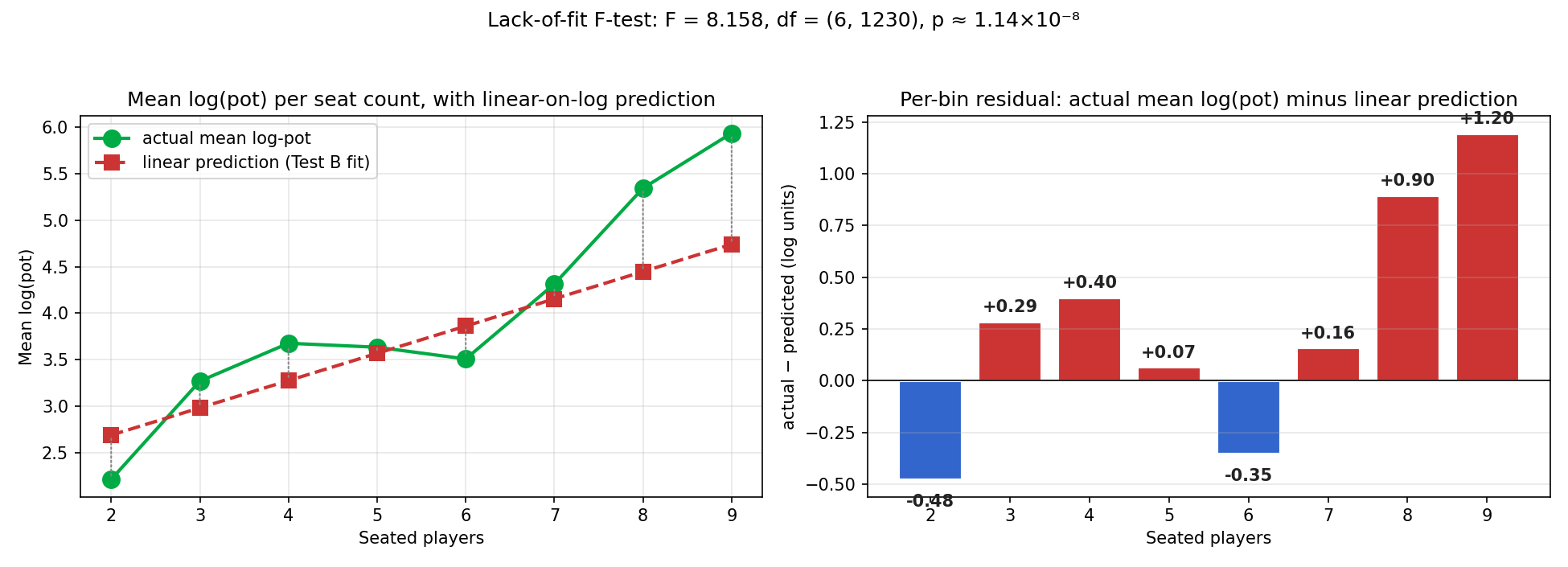
The line under-predicts at 3–4 seats (medium-table action is larger than a line through 2 and 9 would suggest), over-predicts at 6 seats (the modal table is quieter than the line says), and under-predicts dramatically at 8–9 seats (full ring is much wilder than the line says). The gap pattern in the right panel is "wave then explosion" — never noise around zero.

• The test result is partly driven by the 7–9-seat region, where the 85 hands all originate from one table (Aquarium). It is a real signal in the data, but the strength of evidence depends sensitively on whether Aquarium's behavior is representative of full-ring tables in general; this is a substantive concern about generalization that the iid caveats compound.

Putting the three tests together

The analysis started with four candidate tests; three were run and one was dropped for failing its conditions.

Test	What it asks	Statistic	p-value	Decision
Raw OLS slope t-test	linear slope on raw scale	—	—	not run — LINER fails (L, N, E)
A. Chi-square independence	is there any association?	${\chi }^2=111.61$, df $=9$	$6.9\times 10^{-20}$	reject $H_0$ (independence)
B. Log-linear OLS slope	multiplicative slope on log scale	$t=7.24$, df $=1236$	$8.0\times 10^{-13}$	reject $H_0$: ${\beta }_1=0$
C. Lack-of-fit F (log scale)	is the linear-on-log shape right?	$F=8.16$, df $=(6,1230)$	$1.1\times 10^{-8}$	reject $H_0$ (linearity)

Under the iid assumption, the verdict from the three tests run is:

• A: pot size and seat count are not independent; the chi-square cell pattern shows the action is concentrated at the extremes (HU/3-max under-represented in big pots, full ring over-represented in big pots).
• B: the typical pot grows multiplicatively with seat count, by a factor of about $1.34$ per extra seat (95 % CI: $1.24\times$ to $1.45\times$ per seat). Moving from heads-up to 6-max more than triples the typical pot.
• C: the linear-on-log model is not actually the right shape. The fitted log-linear line under-predicts at 3–4 seats and at 8–9 seats and over-predicts at 6 seats. There is more structure than a single multiplicative rate captures.

The independence warning, restated

The independence condition was accepted with a warning at the top: cards deal independently, but within-table behavior carries some correlation. That warning enters the conclusions only as a small upward adjustment to each p-value:

• A's ${\chi }^2=111.61$ might shrink modestly under a cluster-robust correction, but at $p\approx 10^{-20}$ the conclusion "there is some association" is robust to any plausible adjustment.
• B's $p\approx 10^{-13}$ has so much margin that even an order-of-magnitude inflation in $p$ would still leave the slope decisively significant.
• C's $p\approx 10^{-8}$ is heavily driven by the 7–9-seat bins, all from one table (Aquarium). If Aquarium's behavior is unrepresentative of full-ring tables in general, the generalization of the conclusion weakens — a substantive concern distinct from the within-test independence assumption. The 2–6-seat non-linearity, supported by all six tables, is the more robust finding.

What is actually concluded

• Raw-scale linear regression: not entitled. LINER fails on too many fronts. No "$p=0.013$ for the slope on the raw scale" is reported, because the procedure says it shouldn't be.
• An association exists: very likely real. Test A is robust enough ($p\approx 10^{-20}$) to survive any sane correction.
• A multiplicative trend exists: very likely real. Test B's signal ($p\approx 10^{-13}$) is robust enough to survive sizable clustering corrections. The cleanest single-number summary is "each extra seat multiplies the typical pot by roughly $1.34$", treated as an approximation rather than a per-hand prediction.
• A line on the log scale is the wrong model. Test C rejects linearity even after the log transform. The actual per-bin means ($2.21,3.27,3.68,3.63,3.51,4.31,5.34,5.93$ in log-BB at seats 2–9) curve and explode in ways no single slope can capture.

The natural next moves are: (a) collect more tables, not more hands, to break the clustering issue; (b) fit a richer model — a quadratic in seats, a separate intercept per table (mixed-effects), or simply present the per-bin means with proper uncertainty. Those are deferred to a future post.

Materials

Everything used to produce this post is hosted alongside it.

• Dataset — pot-vs-seats-data.zip (359 KB). The CSV bundle from the /data/export-csv endpoint, containing hands.csv, actions.csv, players.csv, and a README. 1238 hands of 1/2 NL Hold'em from 6 tables.
• Main pipeline — pot-vs-seats.py (19 KB). Reproduces every figure and prints every test statistic in this post. Place it next to the data ZIP and run python3 pot-vs-seats.py.
• Arithmetic walkthrough — pot-vs-seats-arith.py (9 KB). Prints every intermediate sum ($\sum x$, $\sum y$, $S_{xx}$, $S_{yy}$, $S_{xy}$, ${\hat{\beta }}_1$, $\mathrm{SSE}$, …) so each by-hand quantity quoted in the post can be verified.

Both scripts depend on pandas, numpy, scipy, statsmodels, and matplotlib. Quickstart:

python3 -m venv .venv && source .venv/bin/activate
pip install pandas numpy scipy statsmodels matplotlib

# Drop the data ZIP next to the scripts, then:
python3 pot-vs-seats.py        # full pipeline (figures + summary)
python3 pot-vs-seats-arith.py  # detailed arithmetic

The whole computation runs in under a second on a modern laptop.

For convenience, both scripts are included verbatim below.

pot-vs-seats.py

The main pipeline. A single main() function calls each test in order and writes every figure used in the post.

#!/usr/bin/env python3
"""
Pot size vs number of seated players — full analysis pipeline.

Reproduces every numerical result and figure used in the blog post
"Does table size drive pot size? A LINER-checked walk through three
tests on 1238 hands":

    https://www.sinostatistica.net/blog/pot-vs-seats-bootstrap

Tests run, in order:
    A.  Chi-square test of independence on a 4 x 4 contingency table.
    B.  Log-linear OLS slope t-test (regress log(pot) on num_seats).
    C.  Lack-of-fit F-test on the log scale (compare linear vs saturated).

A would-be Test 1 (raw OLS slope t-test) is computed for the LINER
diagnostic only and *not reported* as inference, because LINER fails
on the raw scale.

Inputs:   pot-vs-seats-data.zip (the CSV bundle exported from
          /data/export-csv on statisticasino).
Outputs:  fig-*.png in the same directory and stdout summary.

Run:      python3 pot-vs-seats.py
Depends:  pandas, numpy, scipy, statsmodels, matplotlib.
"""
from __future__ import annotations

import io
import zipfile
from pathlib import Path

import matplotlib.pyplot as plt
import numpy as np
import pandas as pd
import statsmodels.api as sm
import statsmodels.formula.api as smf
from scipy.stats import chi2_contingency

# ---------------------------------------------------------------------------
# Configuration
# ---------------------------------------------------------------------------

HERE = Path(__file__).parent
DATA_ZIP = HERE / "pot-vs-seats-data.zip"   # next to this script
OUT = HERE                                  # write figures next to this script
BB = 2                                      # 1/2 NL: big blind = 2 chips
RNG = np.random.default_rng(20260524)       # for jitter on scatter plots


# ---------------------------------------------------------------------------
# Data loading
# ---------------------------------------------------------------------------

def load_bundle(zip_path: Path):
    """Read hands.csv and actions.csv out of the export ZIP."""
    zf = zipfile.ZipFile(zip_path)

    def _read(name):
        member = next(n for n in zf.namelist() if n.endswith(name))
        return pd.read_csv(io.BytesIO(zf.read(member)))

    return _read("hands.csv"), _read("actions.csv")


def build_dataset(hands: pd.DataFrame, actions: pd.DataFrame) -> pd.DataFrame:
    """Aggregate voluntary chips into per-hand pot_BB.

    Voluntary chips = bet + call + raise + allIn (excludes blinds).
    """
    voluntary = (actions
                 .query("action in ['bet','call','raise','allIn'] and chips > 0")
                 .groupby("hand_key")["chips"].sum()
                 .rename("pot_chips"))
    df = (hands.set_index("hand_key")
                .join(voluntary, how="inner")
                .assign(pot_bb=lambda d: d.pot_chips / BB)
                .query("pot_bb > 0 and 2 <= num_seats <= 9")
                .reset_index()
                .sort_values(["table_id", "first_ts"])
                .reset_index(drop=True))
    df["log_pot"] = np.log(df.pot_bb)
    return df


# ---------------------------------------------------------------------------
# Descriptive summary (data tour)
# ---------------------------------------------------------------------------

def descriptive_summary(df: pd.DataFrame) -> None:
    n = len(df)
    print(f"n rounds                : {n}")
    print(f"n distinct tables       : {df.table_id.nunique()}")
    print(f"hands per num_seats     : "
          f"{dict(df.num_seats.value_counts().sort_index())}")
    print(f"pot quartiles (BB)      : "
          f"{df.pot_bb.quantile([.05,.25,.5,.75,.95]).round(1).to_list()}")
    print(f"pot mean / sd  (BB)     : "
          f"{df.pot_bb.mean():.2f} / {df.pot_bb.std():.2f}\n")

    per_table = (df.groupby("table_id")
                   .agg(n_hands=("pot_bb", "size"),
                        seats_min=("num_seats", "min"),
                        seats_max=("num_seats", "max"),
                        seats_modal=("num_seats", lambda s: s.mode().iloc[0]),
                        pot_median=("pot_bb", "median"),
                        pot_mean=("pot_bb", "mean")))
    per_table["table_label"] = (df.groupby("table_id").table_name.first()
                                  .str.replace("Low Stakes - ", "")
                                  .str.replace(" - 1/2 - NL Holdem", ""))
    print("=== Per-table summary ===")
    print(per_table.round(1).to_string(), "\n")
    return per_table


# ---------------------------------------------------------------------------
# Test A — Chi-square test of independence
# ---------------------------------------------------------------------------

def test_a_chi_square(df: pd.DataFrame):
    pot_q = df.pot_bb.quantile([.25, .5, .75]).values
    df["pot_cat"] = pd.cut(df.pot_bb,
                           bins=[-np.inf, *pot_q, np.inf],
                           labels=["tiny", "small", "medium", "big"])
    df["seat_cat"] = pd.cut(df.num_seats,
                            bins=[1, 3, 5, 6, 9],
                            labels=["HU/3", "4-5", "6-max", "full ring"])
    ct = pd.crosstab(df.seat_cat, df.pot_cat)

    chi2, chi_p, chi_dof, chi_exp = chi2_contingency(ct)
    cramers_v = np.sqrt(chi2 / (len(df) * (min(ct.shape) - 1)))

    print("=== Test A: Chi-square test of independence ===")
    print("Observed counts:")
    print(ct.to_string())
    print(f"\n  χ² = {chi2:.2f}, df = {chi_dof}, p = {chi_p:.3g}")
    print(f"  Cramer's V = {cramers_v:.3f}\n")

    return ct, chi_exp, chi2, chi_p, chi_dof, cramers_v


# ---------------------------------------------------------------------------
# Test B — Log-linear OLS slope t-test
# ---------------------------------------------------------------------------

def test_b_log_linear(df: pd.DataFrame):
    fit = smf.ols("log_pot ~ num_seats", data=df).fit()
    b1, se = fit.params["num_seats"], fit.bse["num_seats"]
    print("=== Test B: Log-linear OLS slope t-test ===")
    print(f"  β̂₀ = {fit.params['Intercept']:.4f}, β̂₁ = {b1:.4f}")
    print(f"  SE(β̂₁) = {se:.4f}, "
          f"t = {fit.tvalues['num_seats']:.3f}, "
          f"p = {fit.pvalues['num_seats']:.3g}")
    print(f"  95% CI on β₁ (log)   = "
          f"{fit.conf_int().loc['num_seats'].round(4).to_list()}")
    print(f"  Multiplicative effect e^β̂₁ = {np.exp(b1):.3f} per seat")
    print(f"  HU → 6-max factor    = e^(4·β̂₁) = {np.exp(4*b1):.3f}")
    print(f"  R²                   = {fit.rsquared:.4f}\n")
    return fit


# ---------------------------------------------------------------------------
# Test C — Lack-of-fit F-test on the log scale
# ---------------------------------------------------------------------------

def test_c_lack_of_fit(df: pd.DataFrame, lin_log):
    saturated = smf.ols("log_pot ~ C(num_seats)", data=df).fit()
    table = sm.stats.anova_lm(lin_log, saturated)
    print("=== Test C: Lack-of-fit F-test (log scale) ===")
    print(table.round(4).to_string())
    p = table["Pr(>F)"].iloc[1]
    print(f"\n  lack-of-fit p ≈ {p:.3g}\n")
    return saturated, table


# ---------------------------------------------------------------------------
# Figures
# ---------------------------------------------------------------------------

def fig_hist(df: pd.DataFrame) -> None:
    """Pot-size histogram, linear vs log."""
    fig, (ax1, ax2) = plt.subplots(1, 2, figsize=(11, 4))
    ax1.hist(df.pot_bb, bins=80, color="#888", alpha=0.85, edgecolor="white")
    ax1.set_xlabel("Pot size (BB)")
    ax1.set_ylabel("Hands")
    ax1.set_title(f"Pot size distribution, linear scale "
                  f"(n = {len(df)}, mean = {df.pot_bb.mean():.1f} BB, "
                  f"median = {df.pot_bb.median():.1f} BB)")
    ax2.hist(df.log_pot, bins=60, color="#3a6", alpha=0.85, edgecolor="white")
    ax2.set_xlabel("log(pot size, BB)")
    ax2.set_ylabel("Hands")
    ax2.set_title("Pot size distribution, log scale")
    fig.tight_layout()
    fig.savefig(OUT / "fig-hist.png", dpi=150)


def fig_seat_counts(df: pd.DataFrame) -> None:
    """Bar chart of hand counts per seat-count tier."""
    counts = df.num_seats.value_counts().sort_index()
    fig, ax = plt.subplots(figsize=(9, 4.2))
    ax.bar(counts.index, counts.values,
           color="#5a89c2", edgecolor="white", linewidth=1.5)
    for x, y in zip(counts.index, counts.values):
        ax.text(x, y + 8, str(int(y)), ha="center", va="bottom",
                fontsize=10, color="#234", fontweight="bold")
    ax.set_xlabel("Seated players")
    ax.set_ylabel("Hands")
    ax.set_xticks(range(2, 10))
    ax.set_title(f"Hand counts by seat count (n = {len(df)})")
    ax.grid(alpha=0.3, axis="y")
    ax.set_ylim(0, max(counts.values) * 1.12)
    fig.tight_layout()
    fig.savefig(OUT / "fig-seat-counts.png", dpi=150)


def fig_by_table(df: pd.DataFrame, per_table: pd.DataFrame) -> None:
    """Per-table boxplot of pot sizes (log axis)."""
    n_tables = df.table_id.nunique()
    ordered = per_table.sort_values("n_hands", ascending=False)
    labels = ordered.table_label.tolist()
    boxdata = [df[df.table_id == ordered.index[i]].pot_bb.values
               for i in range(n_tables)]

    fig, ax = plt.subplots(figsize=(9, 4.5))
    bp = ax.boxplot(boxdata, labels=labels, vert=True,
                    patch_artist=True, showfliers=False)
    for patch in bp["boxes"]:
        patch.set_facecolor("#ace")
        patch.set_alpha(0.7)
    ax.set_yscale("log")
    ax.set_ylabel("Pot size (BB, log scale)")
    ax.set_title("Pot size distribution by table (log scale)")
    ax.grid(alpha=0.3, axis="y")
    plt.setp(ax.get_xticklabels(), rotation=15, ha="right")
    fig.tight_layout()
    fig.savefig(OUT / "fig-by-table.png", dpi=150)


def fig_scatter_linear(df: pd.DataFrame, lin_iid) -> None:
    """Linear-Y scatter, clipped at 1200 BB so structure is visible."""
    n = len(df)
    jitter = RNG.uniform(-0.18, 0.18, n)
    xs = np.linspace(df.num_seats.min(), df.num_seats.max(), 100)
    bin_mean = df.groupby("num_seats").pot_bb.mean()
    pred = lin_iid.get_prediction(pd.DataFrame({"num_seats": xs})).summary_frame()

    fig, ax = plt.subplots(figsize=(9, 5.5))
    ax.scatter(df.num_seats + jitter, df.pot_bb,
               alpha=0.10, s=14, color="#444", linewidth=0)
    ax.scatter(bin_mean.index, bin_mean.values,
               color="#0a4", s=110, zorder=5, edgecolor="white",
               linewidth=1.8, label="bin mean")
    ax.plot(xs, pred["mean"], color="#c33", linewidth=2.2,
            label=f"raw OLS line (would-be fit): pot = "
                  f"{lin_iid.params['Intercept']:.1f} + "
                  f"{lin_iid.params['num_seats']:.2f}·seats")
    for k, m in bin_mean.items():
        ax.annotate(f"{m:.0f}", (k, m), xytext=(0, 8),
                    textcoords="offset points", ha="center",
                    fontsize=9, color="#063")
    ax.set_xlabel("Seated players")
    ax.set_ylabel("Voluntary pot contribution (BB)")
    ax.set_ylim(0, 1200)
    ax.set_xticks(range(2, 10))
    ax.set_title("Pot size versus seat count, linear-Y scale "
                 "(Y-axis clipped at 1200 BB)")
    ax.legend(loc="upper left")
    ax.grid(alpha=0.3)
    fig.tight_layout()
    fig.savefig(OUT / "fig-scatter-linear.png", dpi=150)


def fig_scatter_log(df: pd.DataFrame, lin_log) -> None:
    """Log-Y scatter with the log-linear fit."""
    n = len(df)
    jitter = RNG.uniform(-0.18, 0.18, n)
    xs = np.linspace(df.num_seats.min(), df.num_seats.max(), 100)
    bin_geo = np.exp(df.groupby("num_seats").log_pot.mean())
    pred = lin_log.get_prediction(pd.DataFrame({"num_seats": xs})).summary_frame()

    fig, ax = plt.subplots(figsize=(9, 5.5))
    ax.scatter(df.num_seats + jitter, df.pot_bb,
               alpha=0.10, s=14, color="#444", linewidth=0)
    ax.scatter(bin_geo.index, bin_geo.values,
               color="#0a4", s=110, zorder=5, edgecolor="white",
               linewidth=1.8,
               label="bin geometric mean = e^(mean log-pot)")
    ax.plot(xs, np.exp(pred["mean"]), color="#c33", linewidth=2.2,
            label=f"log-linear OLS fit: log(pot) = "
                  f"{lin_log.params['Intercept']:.2f} + "
                  f"{lin_log.params['num_seats']:.3f}·seats")
    ax.fill_between(xs,
                    np.exp(pred["mean_ci_lower"]),
                    np.exp(pred["mean_ci_upper"]),
                    color="#c33", alpha=0.15, label="95% CI band (iid)")
    for k, m in bin_geo.items():
        ax.annotate(f"{m:.0f}", (k, m), xytext=(0, 8),
                    textcoords="offset points", ha="center",
                    fontsize=9, color="#063")
    ax.set_xlabel("Seated players")
    ax.set_ylabel("Voluntary pot contribution (BB, log scale)")
    ax.set_yscale("log")
    ax.set_xticks(range(2, 10))
    ax.set_title("Pot size versus seat count, log-Y scale, "
                 "with log-linear OLS fit and 95% CI band")
    ax.legend(loc="upper left")
    ax.grid(alpha=0.3, which="both")
    fig.tight_layout()
    fig.savefig(OUT / "fig-scatter-log.png", dpi=150)


def fig_chi_square(ct: pd.DataFrame, chi_exp, chi2, chi_p, chi_dof,
                   cramers_v) -> None:
    """3-panel heatmap: observed | expected | per-cell contributions."""
    contrib = (ct.to_numpy() - chi_exp) ** 2 / chi_exp
    panels = [
        ("Observed counts",         ct.to_numpy(), "Blues",  "{:.0f}"),
        ("Expected counts (R·C/N)", chi_exp,       "Greens", "{:.1f}"),
        ("Per-cell (O − E)² / E",   contrib,       "Reds",   "{:.2f}"),
    ]
    seat_lbls = ["HU/3", "4-5", "6-max", "Full ring"]
    pot_lbls = ["tiny", "small", "medium", "big"]

    fig, axes = plt.subplots(1, 3, figsize=(14, 4.4))
    for ax, (title, mat, cmap, fmt) in zip(axes, panels):
        im = ax.imshow(mat, cmap=cmap, aspect="auto")
        ax.set_xticks(range(len(pot_lbls)))
        ax.set_xticklabels(pot_lbls)
        ax.set_yticks(range(len(seat_lbls)))
        ax.set_yticklabels(seat_lbls)
        ax.set_xlabel("pot tier")
        if title.startswith("Observed"):
            ax.set_ylabel("seats tier")
        ax.set_title(title)
        vmax = mat.max()
        for i in range(mat.shape[0]):
            for j in range(mat.shape[1]):
                v = mat[i, j]
                color = "white" if v > 0.55 * vmax else "#222"
                ax.text(j, i, fmt.format(v), ha="center", va="center",
                        color=color, fontsize=10)
        plt.colorbar(im, ax=ax, fraction=0.046, pad=0.04)
    fig.suptitle(f"Chi-square test: χ² = {chi2:.2f}, df = {chi_dof}, "
                 f"p ≈ {chi_p:.1e}, Cramer's V = {cramers_v:.3f}",
                 fontsize=12)
    fig.tight_layout(rect=[0, 0, 1, 0.94])
    fig.savefig(OUT / "fig-chi-square.png", dpi=150)


def fig_within_bin_sd(df: pd.DataFrame) -> None:
    """Per-seat within-bin SD of log(pot) for the equal-variance check."""
    sd = df.groupby("num_seats").log_pot.std().sort_index()
    fig, ax = plt.subplots(figsize=(9, 4.2))
    ax.bar(sd.index, sd.values,
           color="#c8a149", edgecolor="white", linewidth=1.5)
    for x, y in zip(sd.index, sd.values):
        ax.text(x, y + 0.04, f"{y:.2f}", ha="center", va="bottom",
                fontsize=10, color="#5a3", fontweight="bold")
    ax.axhline(sd.min(), color="#666", linestyle="--", linewidth=1,
               label=f"min SD = {sd.min():.2f}")
    ax.axhline(2 * sd.min(), color="red", linestyle="--", linewidth=1,
               label=f"2× min SD = {2*sd.min():.2f} (rule-of-thumb ceiling)")
    ax.set_xlabel("Seated players")
    ax.set_ylabel("Within-bin SD of log(pot)")
    ax.set_xticks(range(2, 10))
    ax.set_ylim(0, max(sd.values) * 1.18)
    ax.set_title("Within-seat standard deviation of log(pot) "
                 "(equal-variance diagnostic)")
    ax.legend(loc="upper right")
    ax.grid(alpha=0.3, axis="y")
    fig.tight_layout()
    fig.savefig(OUT / "fig-within-bin-sd.png", dpi=150)


def fig_bin_means_log(df: pd.DataFrame, lin_log) -> None:
    """Heart of Test C: actual vs linear-predicted log-mean by seat."""
    mean_log = df.groupby("num_seats").log_pot.mean().sort_index()
    seats = mean_log.index.to_numpy()
    pred = lin_log.params["Intercept"] + lin_log.params["num_seats"] * seats
    gap = mean_log.values - pred

    fig, (axL, axR) = plt.subplots(1, 2, figsize=(13, 4.7),
                                    gridspec_kw={"width_ratios": [1, 1]})
    # Left: actual vs predicted
    axL.plot(seats, mean_log.values, "o-", color="#0a4", markersize=10,
             linewidth=2, label="actual mean log-pot")
    axL.plot(seats, pred, "s--", color="#c33", markersize=9,
             linewidth=2, label="linear prediction (Test B fit)")
    for s, m, p in zip(seats, mean_log.values, pred):
        axL.annotate("", xy=(s, m), xytext=(s, p),
                     arrowprops=dict(arrowstyle="-", color="#888",
                                     linestyle=":", linewidth=1))
    axL.set_xlabel("Seated players")
    axL.set_ylabel("Mean log(pot)")
    axL.set_xticks(range(2, 10))
    axL.set_title("Mean log(pot) per seat count, with linear-on-log prediction")
    axL.legend(loc="upper left")
    axL.grid(alpha=0.3)

    # Right: signed gap
    colors = ["#c33" if g > 0 else "#36c" for g in gap]
    axR.bar(seats, gap, color=colors, edgecolor="white", linewidth=1.5)
    for s, g in zip(seats, gap):
        axR.text(s, g + (0.03 if g >= 0 else -0.07), f"{g:+.2f}",
                 ha="center", va="bottom" if g >= 0 else "top",
                 fontsize=10, fontweight="bold", color="#222")
    axR.axhline(0, color="black", linewidth=0.8)
    axR.set_xlabel("Seated players")
    axR.set_ylabel("actual − predicted (log units)")
    axR.set_xticks(range(2, 10))
    axR.set_title("Per-bin residual: actual mean log(pot) minus linear prediction")
    axR.grid(alpha=0.3, axis="y")

    fig.suptitle("Lack-of-fit F-test: F = 8.158, df = (6, 1230), p ≈ 1.14×10⁻⁸", fontsize=12)
    fig.tight_layout(rect=[0, 0, 1, 0.94])
    fig.savefig(OUT / "fig-bin-means-log.png", dpi=150)


# ---------------------------------------------------------------------------
# Main
# ---------------------------------------------------------------------------

def main() -> None:
    hands, actions = load_bundle(DATA_ZIP)
    df = build_dataset(hands, actions)
    per_table = descriptive_summary(df)

    # Raw OLS: fit but DO NOT report inference (LINER fails on raw scale).
    # We only use the fit to draw the would-be OLS line on fig-scatter-linear.
    lin_iid = smf.ols("pot_bb ~ num_seats", data=df).fit()

    ct, chi_exp, chi2, chi_p, chi_dof, cramers_v = test_a_chi_square(df)
    lin_log = test_b_log_linear(df)
    sat_log, lof_table = test_c_lack_of_fit(df, lin_log)

    fig_hist(df)
    fig_seat_counts(df)
    fig_by_table(df, per_table)
    fig_scatter_linear(df, lin_iid)
    fig_scatter_log(df, lin_log)
    fig_chi_square(ct, chi_exp, chi2, chi_p, chi_dof, cramers_v)
    fig_within_bin_sd(df)
    fig_bin_means_log(df, lin_log)

    print("All figures written to:", OUT)


if __name__ == "__main__":
    main()

pot-vs-seats-arith.py

The arithmetic walkthrough. Print every intermediate sum that goes into each formula, exactly as quoted in the post.

#!/usr/bin/env python3
"""
Pot size vs number of seated players — arithmetic walkthrough.

Companion to pot-vs-seats.py. Where the main script just calls the
high-level statsmodels routines and prints the results, this script
prints every intermediate quantity that the blog post plugs into a
formula by hand:

    Test 1 (raw OLS, dropped):  Σx, Σy, Σx², Σy², Σxy, Sxx, Syy, Sxy,
                                β̂₀, β̂₁, SSE, R², s, SE, t, p, CI.
    Test B (log OLS):            same set, on the log scale.
    Test C (lack-of-fit F):      SSE_lin, SSE_sat, df, MS_LoF, MS_PE, F, p.
    Test A (chi-square):         observed table, row/col totals, expected
                                 table, per-cell (O−E)²/E, χ², df, p,
                                 Cramer's V.

Run:      python3 pot-vs-seats-arith.py
Inputs:   pot-vs-seats-data.zip (next to this script)
Depends:  pandas, numpy, scipy, statsmodels.
"""
from __future__ import annotations

import io
import zipfile
from pathlib import Path

import numpy as np
import pandas as pd
import statsmodels.api as sm
import statsmodels.formula.api as smf
from scipy.stats import chi2 as chi2_dist
from scipy.stats import f as f_dist
from scipy.stats import t as student_t

HERE = Path(__file__).parent
DATA_ZIP = HERE / "pot-vs-seats-data.zip"
BB = 2


# ---------------------------------------------------------------------------
# Data loading
# ---------------------------------------------------------------------------

zf = zipfile.ZipFile(DATA_ZIP)


def _read(name: str) -> pd.DataFrame:
    member = next(n for n in zf.namelist() if n.endswith(name))
    return pd.read_csv(io.BytesIO(zf.read(member)))


hands = _read("hands.csv")
actions = _read("actions.csv")
voluntary = (actions
             .query("action in ['bet','call','raise','allIn'] and chips > 0")
             .groupby("hand_key")["chips"].sum()
             .rename("pot_chips"))
df = (hands.set_index("hand_key").join(voluntary, how="inner")
            .assign(pot_bb=lambda d: d.pot_chips / BB)
            .query("pot_bb > 0 and 2 <= num_seats <= 9")
            .reset_index())

n = len(df)
x = df.num_seats.to_numpy().astype(float)
y = df.pot_bb.to_numpy().astype(float)


# ---------------------------------------------------------------------------
# Shared X-related sums
# ---------------------------------------------------------------------------

xbar = x.mean()
ybar = y.mean()
Sxx = ((x - xbar) ** 2).sum()
Syy = ((y - ybar) ** 2).sum()
Sxy = ((x - xbar) * (y - ybar)).sum()


# ===========================================================================
# Test 1 (raw OLS, dropped: LINER fails)
# ---------------------------------------------------------------------------
# We compute these only to display the would-be OLS line on the linear
# scatterplot. They are NOT reported as inference.
# ===========================================================================

beta1 = Sxy / Sxx
beta0 = ybar - beta1 * xbar
yhat = beta0 + beta1 * x
SSE = ((y - yhat) ** 2).sum()
SST = Syy
SSR_model = SST - SSE
R2 = 1 - SSE / SST
s2 = SSE / (n - 2)
s = np.sqrt(s2)
SE_b1 = s / np.sqrt(Sxx)
t_stat = beta1 / SE_b1
df_resid = n - 2
p_two = 2 * (1 - student_t.cdf(abs(t_stat), df_resid))
tstar = student_t.ppf(0.975, df_resid)
ci = (beta1 - tstar * SE_b1, beta1 + tstar * SE_b1)

print("=== Raw OLS arithmetic (DROPPED: LINER fails on raw scale) ===")
print(f"n        = {n}")
print(f"x̄       = {xbar:.6f}")
print(f"ȳ       = {ybar:.6f}")
print(f"Σx       = {x.sum():.4f}")
print(f"Σy       = {y.sum():.4f}")
print(f"Σx²      = {(x**2).sum():.4f}")
print(f"Σy²      = {(y**2).sum():.4f}")
print(f"Σxy      = {(x*y).sum():.4f}")
print(f"Sxx      = Σ(x−x̄)²     = {Sxx:.4f}")
print(f"Syy=SST  = Σ(y−ȳ)²     = {Syy:.4f}")
print(f"Sxy      = Σ(x−x̄)(y−ȳ) = {Sxy:.4f}")
print(f"β̂₁      = Sxy / Sxx    = {beta1:.6f}")
print(f"β̂₀      = ȳ − β̂₁·x̄   = {beta0:.6f}")
print(f"SSE      = Σ(y−ŷ)²    = {SSE:.4f}")
print(f"SSR      = SST − SSE   = {SSR_model:.4f}")
print(f"R²       = SSR / SST   = {R2:.6f}")
print(f"s²       = SSE / (n−2) = {s2:.4f}")
print(f"s        = √s²         = {s:.4f}")
print(f"SE(β̂₁)  = s / √Sxx    = {SE_b1:.6f}")
print(f"t        = β̂₁ / SE    = {t_stat:.4f}")
print(f"df_resid = n − 2       = {df_resid}")
print(f"two-sided p (descriptive only) = {p_two:.4g}")
print(f"t*(0.975, {df_resid}) = {tstar:.4f}")
print(f"95% CI on β₁ (descriptive) = "
      f"[{ci[0]:.4f}, {ci[1]:.4f}]\n")


# ===========================================================================
# Test B — Log-linear OLS slope t-test
# ===========================================================================

ly = np.log(y)
ly_bar = ly.mean()
Sllog = ((ly - ly_bar) ** 2).sum()
Sxlog = ((x - xbar) * (ly - ly_bar)).sum()
b1_log = Sxlog / Sxx
b0_log = ly_bar - b1_log * xbar
yhat_log = b0_log + b1_log * x
SSE_log = ((ly - yhat_log) ** 2).sum()
s2_log = SSE_log / (n - 2)
s_log = np.sqrt(s2_log)
SE_b1_log = s_log / np.sqrt(Sxx)
t_log = b1_log / SE_b1_log
p_log = 2 * (1 - student_t.cdf(abs(t_log), df_resid))
ci_log = (b1_log - tstar * SE_b1_log, b1_log + tstar * SE_b1_log)
R2_log = 1 - SSE_log / Sllog

print("=== Test B: Log-linear OLS arithmetic ===")
print(f"ℓ̄         = mean log(y)         = {ly_bar:.6f}")
print(f"Sℓℓ        = Σ(ℓ−ℓ̄)²            = {Sllog:.4f}")
print(f"Sxℓ        = Σ(x−x̄)(ℓ−ℓ̄)       = {Sxlog:.4f}")
print(f"β̂₁_log    = Sxℓ / Sxx           = {b1_log:.6f}")
print(f"β̂₀_log    = ℓ̄ − β̂₁_log · x̄    = {b0_log:.6f}")
print(f"SSE_log    = Σ(ℓ−ℓ̂)²            = {SSE_log:.4f}")
print(f"s²_log     = SSE/(n−2)            = {s2_log:.6f}")
print(f"s_log      = √s²                  = {s_log:.6f}")
print(f"SE(β̂₁_log)= s_log / √Sxx         = {SE_b1_log:.6f}")
print(f"t_log      = β̂₁_log / SE         = {t_log:.4f}")
print(f"two-sided p_log                    = {p_log:.4g}")
print(f"95% CI on β₁_log                   = "
      f"[{ci_log[0]:.4f}, {ci_log[1]:.4f}]")
print(f"e^β̂₁_log   = ×{np.exp(b1_log):.4f} per seat")
print(f"e^(4·β̂₁)   = ×{np.exp(4*b1_log):.4f}  (HU→6-max)")
print(f"R²_log     = {R2_log:.4f}\n")


# ===========================================================================
# Test C — Lack-of-fit F-test (log scale)
# ===========================================================================

lin_log_fit = smf.ols("np.log(pot_bb) ~ num_seats", data=df).fit()
sat_log_fit = smf.ols("np.log(pot_bb) ~ C(num_seats)", data=df).fit()
SSE_lin_log = lin_log_fit.ssr
SSE_sat_log = sat_log_fit.ssr
df_lin = lin_log_fit.df_resid
df_sat = sat_log_fit.df_resid
df_diff = df_lin - df_sat
SS_diff = SSE_lin_log - SSE_sat_log
MS_LoF = SS_diff / df_diff
MS_PE = SSE_sat_log / df_sat
F = MS_LoF / MS_PE
p_F = 1 - f_dist.cdf(F, df_diff, df_sat)

print("=== Test C: Lack-of-fit F arithmetic (log scale) ===")
print(f"SSE_lin_log = {SSE_lin_log:.4f},  df_lin = {df_lin}")
print(f"SSE_sat_log = {SSE_sat_log:.4f},  df_sat = {df_sat}")
print(f"df_diff     = df_lin − df_sat       = {df_diff}")
print(f"SS_diff     = SSE_lin − SSE_sat     = {SS_diff:.4f}")
print(f"MS_LoF      = SS_diff / df_diff     = {MS_LoF:.4f}")
print(f"MS_PE       = SSE_sat / df_sat      = {MS_PE:.4f}")
print(f"F           = MS_LoF / MS_PE        = {F:.4f}")
print(f"p(F > {F:.2f}, df=({df_diff}, {df_sat})) = {p_F:.4g}\n")

print("Per num_seats bin (log scale):")
print(df.groupby("num_seats")
        .agg(n=("pot_bb", "size"),
             mean_log_pot=("pot_bb", lambda v: np.log(v).mean()),
             sd_log_pot=("pot_bb", lambda v: np.log(v).std()))
        .round(4).to_string())
print()


# ===========================================================================
# Test A — Chi-square test of independence
# ===========================================================================

df["pot_cat"] = pd.qcut(df.pot_bb, 4, labels=["tiny", "small", "medium", "big"])
df["seat_cat"] = pd.cut(df.num_seats, bins=[1, 3, 5, 6, 9],
                        labels=["HU/3", "4-5", "6-max", "full ring"])
ct = pd.crosstab(df.seat_cat, df.pot_cat)

row_tot = ct.sum(axis=1).to_numpy()
col_tot = ct.sum(axis=0).to_numpy()
N = ct.sum().sum()
exp = np.outer(row_tot, col_tot) / N
exp_df = pd.DataFrame(exp, index=ct.index, columns=ct.columns)
contrib = (ct.to_numpy() - exp) ** 2 / exp
contrib_df = pd.DataFrame(contrib, index=ct.index, columns=ct.columns)
chi2_stat = contrib.sum()
df_chi = (ct.shape[0] - 1) * (ct.shape[1] - 1)
p_chi = 1 - chi2_dist.cdf(chi2_stat, df_chi)
cramers_v = np.sqrt(chi2_stat / (N * (min(ct.shape) - 1)))

print("=== Test A: Chi-square arithmetic ===")
print("Observed counts:")
print(ct.to_string())
print("\nExpected counts (Rᵢ · Cⱼ / N):")
print(exp_df.round(3).to_string())
print("\nPer-cell (O − E)² / E:")
print(contrib_df.round(3).to_string())
print(f"\nRow sums of contributions: "
      f"{[round(s, 3) for s in contrib.sum(axis=1).tolist()]}")
print(f"Total χ²                  = {chi2_stat:.4f}")
print(f"df = (r−1)(c−1)           = {df_chi}")
print(f"p (χ²_{df_chi} > {chi2_stat:.2f})  = {p_chi:.4e}")
print(f"Cramer's V                 = {cramers_v:.4f}")