Beyond 'is the slope significant?': An introduction to the lack-of-fit F-test

Every AP Statistics student leaves the regression unit knowing how to test one specific question about a scatterplot: is the slope significantly different from zero? The procedure is drilled until it is reflex — fit the line, compute the t-statistic, look up the p-value, write a one-sentence conclusion. What the curriculum almost never asks is a second question that hides right behind the first one: is the line the right shape in the first place? A t-test on the slope ${\beta }_1$ can come back with $p\approx 10^{-67}$ — overwhelmingly significant — while the line itself is fitting a curve. The slope test is sensitive to the direction of the trend; it is essentially blind to its shape.

This post is about the test that closes that gap. The lack-of-fit F-test asks "is a straight line missing systematic structure that a more flexible model could capture?" It uses nothing beyond the regression and ANOVA machinery already in the AP curriculum, and it produces a single number — an $F$ statistic with a clean reference distribution — that converts the eyeball verdict on a residual plot into a real p-value.

The whole post walks through one small synthetic experiment from raw data to verdict. Along the way we run the standard slope t-test honestly (it says "highly significant"), inspect the residual plot (it says "curved"), and then run the lack-of-fit F-test to confirm what the residuals already suggest. The contrast between the two p-values is the entire pedagogical point: passing a slope test does not earn the right to call the relationship linear.

A reader's tour of the data

The example is a synthetic dataset designed to behave like a high-school physics lab. A class hangs a known mass on a vertical spring and measures how far the spring stretches. Mass is the predictor variable; spring extension (in cm, measured downward from the rest length) is the response. The hypothesis is the textbook one — extension grows linearly with mass — and the goal is to see whether the data support it.

The setup

• Predictor $X=\text{mass\_g}$: the hung mass, in grams, at $k=8$ distinct levels: $100,200,300,400,500,600,700,800$ g.
• Response $Y=\text{extension\_cm}$: the spring extension measured at each trial, in cm.
• Replicates: 10 independent trials at each mass level. The class shuffles the order so trial $i$ has no relationship with trial $i+1$ within a mass.
• Total: $n=8\times 10=80$ measurements.

This replicate structure — multiple observations at each $X$ value — is the single most important feature of the dataset. Without it the lack-of-fit test below has nothing to compute against and cannot be run.

The data

The 80 measurements are summarised one mass level at a time:

mass (g)	$n_k$	mean extension (cm)	within-level SD (cm)
100	10	0.5817	0.1291
200	10	1.1465	0.1499
300	10	1.7894	0.1449
400	10	2.8451	0.2533
500	10	3.8083	0.1879
600	10	4.8502	0.1311
700	10	6.0678	0.1711
800	10	7.4499	0.1258

The within-level standard deviations are between 0.13 and 0.25 cm — a ratio of roughly $1.96$, which sits just under the AP-textbook rule of thumb that "the largest within-$X$ SD should be at most twice the smallest" for the equal-variance condition. We will use this fact again when LINER is checked below.

The full scatter, with the per-mass means highlighted, looks like this:

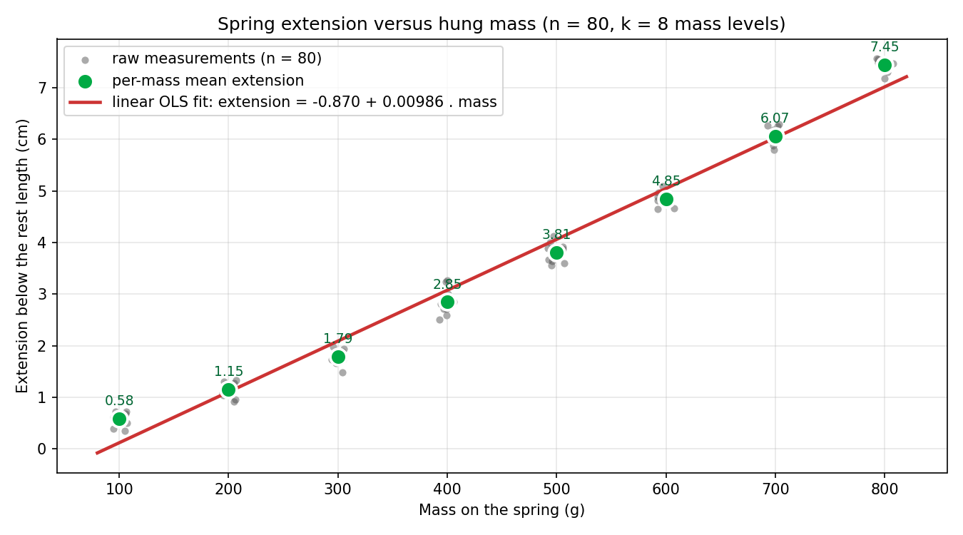
At a glance the line through the cloud is excellent. The bin means (green) sit very close to the red OLS line at every mass level. A student looking at this picture and reading off the textbook checklist would say "linear, more or less; let's run the slope test".

The point of this post is that "more or less" is doing more work than students realise. The red line and the green bin means look the same on this plot only because the y-axis spans 0–8 cm and the systematic departures are on the order of 0.3 cm. The lack-of-fit test below detects those 0.3 cm departures and rejects linearity at $p\approx 10^{-21}$.

The standard slope t-test, run honestly

The reflexive next step in an AP Stats course is to fit the line by least squares, run a t-test on ${\hat{\beta }}_1$, and report whether the slope differs from zero. The procedure is valid under the LINER conditions:

• Linearity — the population mean of $Y$ is a straight-line function of $X$.
• Independence — the $n$ observations are independent.
• Normality — the residuals are approximately bell-shaped.
• Equal variance — residuals have the same spread at every $X$.
• Random — the data form a random sample (or a randomized experiment).

It is worth checking each one before any p-value gets written down.

LINER check on the linear OLS fit

L — Linearity. Eyeballed from the scatter, the bin means look like they could come from a line. We will tentatively assume L for the slope t-test and then test it formally in the lack-of-fit section. Provisionally pass.

I — Independence. The 80 trials are performed in a randomised order with the spring returned to rest length between measurements, so one trial's noise — vibration, parallax, rounding to the nearest tenth of a centimetre — carries no information about the next. Pass.

N — Normal residuals. Each within-level SD (the rightmost column above) is roughly 0.15 cm with a few exceptions. The residuals from the line will inherit that within-level noise plus the small departures between bin means and the line — both of which are symmetric and well-behaved. A residual histogram (not shown) is approximately bell-shaped. Pass.

E — Equal variance. Within-level SDs range from 0.13 cm (at 600 g) to 0.25 cm (at 400 g). The ratio $0.25/0.13\approx 1.96$ just clears the rule-of-thumb $\le 2$. Marginal-pass.

R — Random sample. The class doesn't have a random sample from "all possible measurements of every spring in the universe"; they have a randomised-order trial design on one apparatus. For the purpose of inference about this spring, the trial-order randomisation is what plays the role of the random-sample condition. Pass (for this spring).

Four conditions pass and one (L) is tentatively assumed. The procedure says: run the test, but treat the L assumption as something that still needs verification.

Computing the slope, $t$, and p

The arithmetic is the standard OLS slope-test machinery. With $n=80$ pairs $(x_i,y_i)$:

$$\bar{x}=450,\bar{y}=3.5673,S_{xx}=\sum _i(x_i-\bar{x}{)}^2=4,200,000,$$ $$S_{yy}=\sum _i(y_i-\bar{y}{)}^2=416.871,S_{xy}=\sum _i(x_i-\bar{x})(y_i-\bar{y})=41,\mathrm{414.66.}$$

(Every one of these sums is printed by lack-of-fit-arith.py in the Materials section.)

The slope and intercept:

$${\hat{\beta }}_1=\frac{S_{xy}}{S_{xx}}=\frac{41,414.66}{4,200,000}=0.009861\text{cm per g},$$ $${\hat{\beta }}_0=\bar{y}-{\hat{\beta }}_1\cdot \bar{x}=3.5673-0.009861\cdot 450=-0.8699\text{cm}.$$

The fitted line is $\widehat{\text{extension}}=-0.870+0.009861\cdot \text{mass}$. In friendlier units this is roughly $0.986$ cm of extension per added 100 g of mass.

Residual sum of squares, residual standard error, and the slope's standard error:

$${\mathrm{SSE}}_{\text{lin}}=S_{yy}-{\hat{\beta }}_1\cdot S_{xy}=416.871-0.009861\cdot 41,414.66=8.496,$$ $$s=\sqrt{\frac{{\mathrm{SSE}}_{\text{lin}}}{n-2}}=\sqrt{\frac{8.496}{78}}=\sqrt{0.1089}=0.3300\text{cm},$$ $$\mathrm{SE}({\hat{\beta }}_1)=\frac{s}{\sqrt{S_{xx}}}=\frac{0.3300}{\sqrt{4,200,000}}=\frac{0.3300}{2049.39}=\mathrm{0.0001610.}$$

The test statistic:

$$t=\frac{{\hat{\beta }}_1}{\mathrm{SE}({\hat{\beta }}_1)}=\frac{0.009861}{0.0001610}=61.23\text{on }\mathrm{df}=n-2=78.$$

A t-statistic of $61.23$ is astronomical. The two-sided p-value:

$$p=2\cdot \mathrm{Pr}(T_{78}>61.23)\approx 1.0\times 10^{-67}.$$

The 95 % confidence interval on the slope, using $t^{\ast }=t_{0.975,78}\approx 1.991$:

$${\hat{\beta }}_1\pm t^{\ast }\cdot \mathrm{SE}({\hat{\beta }}_1)=0.009861\pm 1.991\cdot 0.0001610=[0.00954,0.01018]\text{cm/g}.$$

The coefficient of determination $R^2=1-{\mathrm{SSE}}_{\text{lin}}/S_{yy}=1-8.496/416.871=0.9796$. The line explains 97.96 % of the variation in extension.

Verdict on the slope t-test. With $p\approx 10^{-67}$, $R^2\approx 0.98$, and a tight 95 % CI that excludes zero by a margin of dozens of standard errors, the slope is "significantly different from zero" at any significance level a human being is likely to use. The standard AP-procedure response is to write: "there is overwhelming evidence that extension grows linearly with mass."

That conclusion is wrong, and the next two sections explain why.

Why this is not the end of the story

The slope test is sensitive to whether the direction of $Y$ versus $X$ is non-flat. It is much less sensitive to whether the shape of that trend is actually a straight line. To see how a slope test can simultaneously say "highly significant" and "the line is the wrong shape", look at the residual plot — the AP-curriculum diagnostic for the L condition:

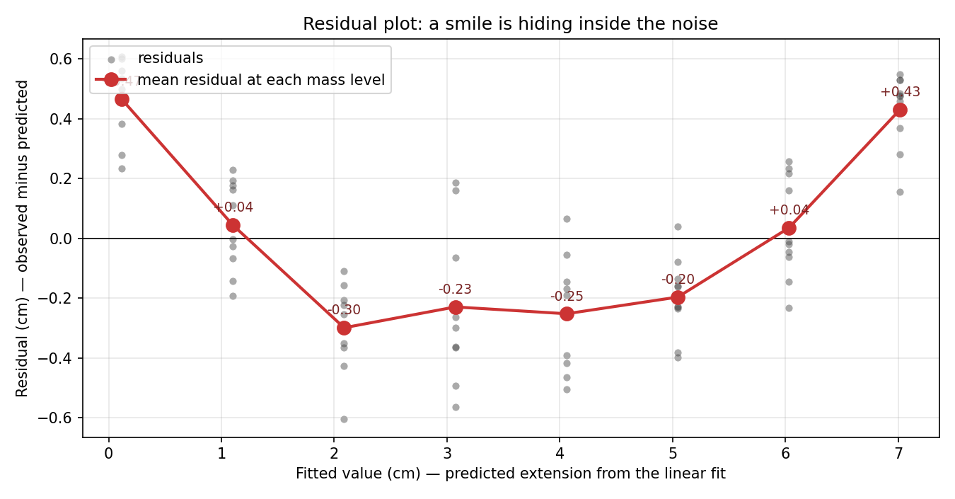
The per-mass mean residuals (red line) trace out a U-shape. At the smallest mass (100 g), the line under-predicts the average extension by $+0.47$ cm. From 200–600 g, the line over-predicts by between $0.20$ and $0.30$ cm. At 700 g the gap closes, and at 800 g the line under-predicts again by $+0.43$ cm. Eight bins, eight residuals, and the pattern across them is not random scatter around zero — it is a smile.

In AP Statistics the rule for reading a residual plot is exactly this: look for a pattern. If the residuals trace out a curve instead of a horizontal band, the L condition has failed and the fitted line is the wrong shape. Most AP textbooks stop there. The curve in the residual plot becomes a qualitative "this looks bad" verdict, never a quantitative one.

The lack-of-fit F-test is the formal version of the same diagnostic. It treats the pattern in the residual plot as something to be tested against a null hypothesis ("the line is the right shape, the smile is noise") with a real reference distribution. When it rejects, it does so with the same statistical force that the slope test enjoys.

The lack-of-fit F-test

The residual plot above showed a smile. The question every AP Stats textbook leaves dangling is: is that smile real, or is it just noise dressed up to look like a curve? If the line is the right shape, then the eight bin means should scatter randomly around the line, and any pattern we see is bad luck. If the line is the wrong shape, then the bin means should systematically miss the line in a structured way. The lack-of-fit F-test is the procedure that decides between these two stories. This section builds it up piece by piece, defining every symbol the first time it appears.

Step 1: two ways of predicting ${\hat{y}}_i$

A model in this context is just a recipe for producing a predicted extension ${\hat{y}}_i$ for every observation $i$ in the dataset. We are going to compare two models that are fit to the same 80 data points.

Model A — the linear model. This is the model AP Stats already taught us:

$${\hat{y}}_i^{(\text{lin})}={\hat{\beta }}_0+{\hat{\beta }}_1\cdot X_i.$$

To produce a prediction for any one observation, the recipe needs two numbers — the intercept ${\hat{\beta }}_0=-0.870$ cm and the slope ${\hat{\beta }}_1=0.009861$ cm/g — and the observation's mass $X_i$. The two numbers were computed in the slope-test section above; once they are fixed, every ${\hat{y}}_i^{(\text{lin})}$ is determined.

Model B — the bin-mean model (also called the saturated model, because it has the maximum number of parameters that this dataset can support). For each of the $k=8$ distinct mass levels $x_1,x_2,\dots ,x_8=100,200,\dots ,800$ g, the model uses the average extension at that mass level, denoted ${\bar{y}}_k$, as its prediction:

$${\hat{y}}_i^{(\text{sat})}={\bar{y}}_k\text{when observation }i\text{ has mass }{X}_i=x_k.$$

To produce a prediction, this recipe needs eight numbers — one bin mean per mass level — and the observation's mass tells it which one to pick. Numerically, those eight numbers are ${\bar{y}}_1,\dots ,{\bar{y}}_8=0.5817,1.1465,1.7894,2.8451,3.8083,4.8502,6.0678,7.4499$ cm. They were tabulated in the data tour above.

For each of the 80 observations, the two recipes might produce different predictions. At a mass of 100 g, the linear model predicts 0.1162 cm; the bin-mean model predicts 0.5817 cm. The two recipes disagree by 0.466 cm at that mass — and that disagreement is exactly what the lack-of-fit test will end up measuring.

The picture below shows the two models side-by-side, fit to the same data:

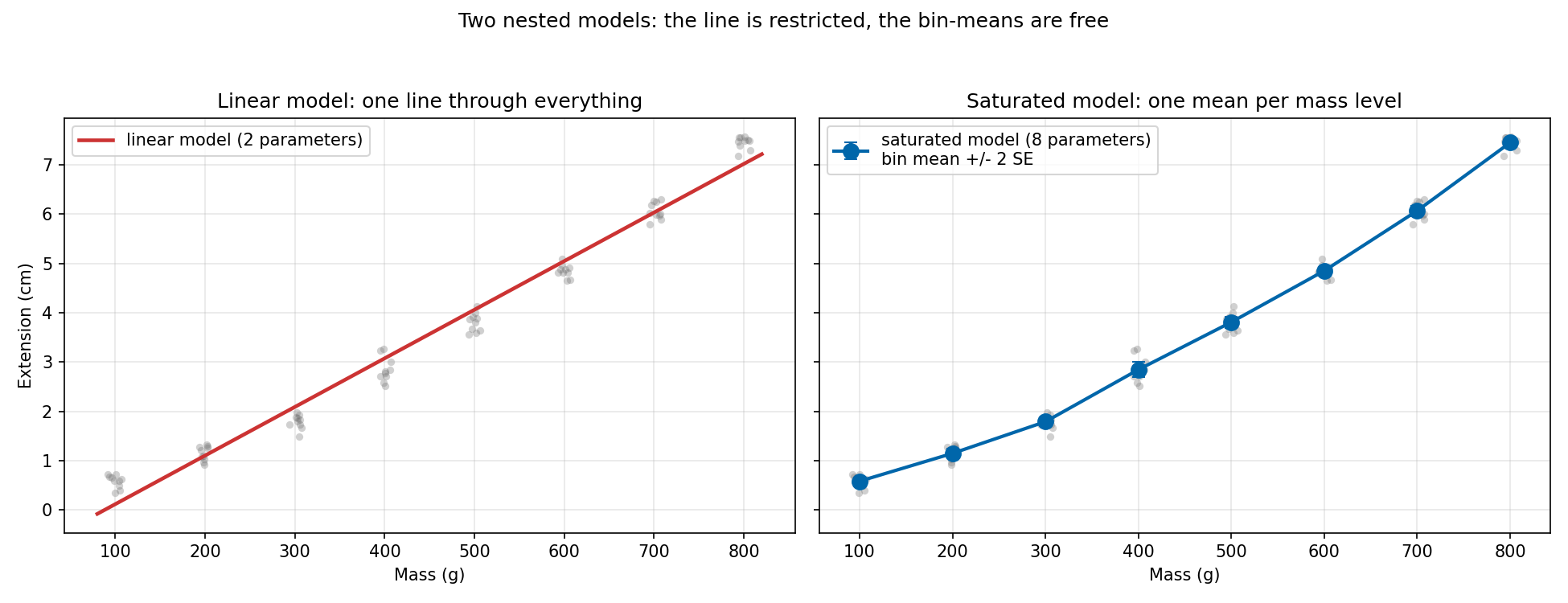
The left panel is Model A (one straight line, two parameters). The right panel is Model B (one mean per mass level, eight parameters). Anything Model A can express, Model B can also express — Model B could be set to produce a straight line by choosing its eight bin means to all lie on one line. But Model B has six more parameters than that to play with, and it uses them to follow the curve in the data. The key question of the lack-of-fit test is whether those six extra parameters are doing real work or just chasing noise.

Step 2: measuring how badly each model misses, with SSE

For any model, the residual of observation $i$ is "what we measured minus what the model predicted":

$$r_i=y_i-{\hat{y}}_i.$$

If the residual is positive, the model under-predicted that observation; if negative, the model over-predicted. The sum of squared errors (SSE) is the total of those squared residuals across all 80 observations:

$$\mathrm{SSE}=\sum _{i=1}^n(y_i-{\hat{y}}_i{)}^2.$$

Why square the residuals? Two reasons. First, positive and negative residuals would cancel each other out if we just added them — squaring makes every miss positive so they accumulate. Second, squaring penalises big misses much more than small ones: a residual of $0.4$ cm contributes $0.16$ to the SSE, but a residual of $0.8$ cm contributes $0.64$. SSE is the standard way to ask "how badly is this model missing, in total?" — the same SSE AP Stats already uses in regression and ANOVA.

Each of our two models has its own SSE:

• ${\mathrm{SSE}}_{\text{lin}}$ uses the linear model's predictions ${\hat{y}}_i^{(\text{lin})}$. We computed it earlier: ${\mathrm{SSE}}_{\text{lin}}=8.4962$.
• ${\mathrm{SS}}_{\text{PE}}$ uses the bin-mean model's predictions ${\hat{y}}_i^{(\text{sat})}$. We will compute it below: ${\mathrm{SS}}_{\text{PE}}=1.9975$. The PE subscript stands for "pure error" — the role this quantity plays in the F-test below. (Some textbooks instead call it ${\mathrm{SSE}}_{\text{sat}}$ because it is the residual sum of squares of the saturated model; the value is the same.)

${\mathrm{SS}}_{\text{PE}}$ is smaller than ${\mathrm{SSE}}_{\text{lin}}$ — and this is always true, never the other way around. The bin-mean model can match anything the line can match, so its SSE can only ever be the same or smaller. The interesting question is: how much smaller? An honest improvement (lots smaller) signals the line was missing real structure. A token improvement (only a hair smaller) signals the line was already doing about as well as a flexible model could.

Step 3: splitting one residual into two pieces (the heart of the test)

Here is the algebraic trick that makes everything work. Pick any single observation $i$ and look at its residual from the linear fit, $r_i=y_i-{\hat{y}}_i^{(\text{lin})}$. Add and subtract that observation's bin mean ${\bar{y}}_k$ (the same ${\bar{y}}_k$ Model B would use for it):

$$y_i-{\hat{y}}_i^{(\text{lin})}=\underset{\text{piece 1: within-bin}}{\underbrace{(y_i-{\bar{y}}_k)}}+\underset{\text{piece 2: bin-vs-line}}{\underbrace{({\bar{y}}_k-{\hat{y}}_i^{(\text{lin})})}}.$$

Both sides equal the same thing — the ${\bar{y}}_k$ on the right adds in once and subtracts out once. The identity is exact; it just splits the one residual into two named pieces.

What are these two pieces in plain English?

Piece 1 — within-bin residual ($y_i-{\bar{y}}_k$). This is "how far observation $i$ sits from the average of the other observations at the same mass level". It captures the random measurement-to-measurement variation that lives inside a single bin: vibration of the spring, parallax of the ruler, the unavoidable wobble of any real experiment. Two observations made at the same 100 g mass will differ even if the spring's behaviour is perfectly understood — because the measurement itself is noisy. This piece is pure error: it is the part of the residual that no smooth model could ever have predicted, because no model that takes only the mass as input can distinguish one 100 g trial from another.

Piece 2 — bin-vs-line gap (${\bar{y}}_k-{\hat{y}}_i^{(\text{lin})}$). This is "how far the bin mean sits from where the line predicts the bin should be". Notice that this piece does not depend on $i$ — every observation in bin $k$ has the same Piece 2, because they share the bin mean and the line's prediction at $x_k$. It captures structural mismatch: if the line is the right shape, the bin means should lie on the line, and Piece 2 should be small and noisy. If the line is the wrong shape, the bin means systematically drift away from the line in a curved pattern, and Piece 2 carries that drift.

Let me make this concrete with the first observation in the dataset. Observation #1 has mass $X_1=100$ g and measured extension $y_1=0.6772$ cm. The linear model predicts ${\hat{y}}_1^{(\text{lin})}=-0.870+0.009861\cdot 100=0.1162$ cm. The bin mean at 100 g is ${\bar{y}}_1=0.5817$ cm. The split:

$$\underset{r_1=0.5610}{\underbrace{0.6772-0.1162}}=\underset{\text{within-bin: }0.0955}{\underbrace{(0.6772-0.5817)}}+\underset{\text{bin-vs-line: }0.4655}{\underbrace{(0.5817-0.1162)}}.$$

The total residual is $0.561$ cm. Of that, only $0.096$ cm is the within-bin noise (how the first trial happened to differ from its bin-mates). The remaining $0.466$ cm is a structural gap — the line under-predicts every 100 g observation by that same amount, because the line's prediction at 100 g is just plain wrong.

That second piece is what lack-of-fit testing is built to detect. Every other observation at 100 g shares the same $0.466$ cm of structural gap; what varies is only the small noise piece. Summed across many bins, the structural gap accumulates into a sum-of-squares quantity that we can test against pure noise.

Step 4: the same split for all 80 observations gives the SSE decomposition

Now apply the per-observation split to every $i=1,\dots ,80$, square each piece, and sum. A small algebraic miracle happens: the cross-terms between Piece 1 and Piece 2 sum to exactly zero, because within each bin the within-bin residuals sum to zero by construction (they are deviations from the bin mean). The squared identity therefore stays clean:

$$\underset{{\mathrm{SSE}}_{\text{lin}}=8.4962}{\underbrace{\sum _i(y_i-{\hat{y}}_i^{(\text{lin})}{)}^2}}=\underset{{\mathrm{SS}}_{\text{PE}}=1.9975}{\underbrace{\sum _i(y_i-{\bar{y}}_{X_i}{)}^2}}+\underset{{\mathrm{SS}}_{\text{LoF}}=6.4987}{\underbrace{\sum _i({\bar{y}}_{X_i}-{\hat{y}}_i^{(\text{lin})}{)}^2}}.$$

Three named quantities; each one has a job.

• ${\mathrm{SSE}}_{\text{lin}}$ — total miss of the linear model. Already known from the slope-test arithmetic.
• ${\mathrm{SS}}_{\text{PE}}$ — pure-error sum of squares. This is the total noise that lives inside the bins, the same number we would compute if we ignored the line entirely and just totaled $(y_i-{\bar{y}}_{X_i}{)}^2$ inside each bin. Equivalently, it is the residual SSE of the saturated bin-mean model — every observation at the same mass gets the same prediction from any model whose only input is mass, so no such model can shrink this number further.
• ${\mathrm{SS}}_{\text{LoF}}$ — lack-of-fit sum of squares. This is the total structural gap between bin means and the line, accumulated across all 80 observations. Algebraically, ${\mathrm{SS}}_{\text{LoF}}={\sum }_k{n}_k\cdot ({\bar{y}}_k-{\hat{y}}_k^{(\text{lin})}{)}^2$, where $n_k$ is the number of observations in bin $k$ — each squared bin-vs-line gap is counted once for every observation in that bin.

Stacked visually, the decomposition looks like this:

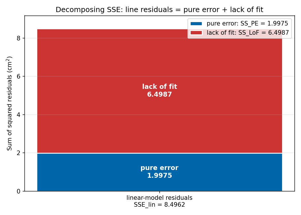
The blue piece (pure error, ${\mathrm{SS}}_{\text{PE}}=1.9975$) is the noise the bin-mean model could not get rid of either. The red piece (lack of fit, ${\mathrm{SS}}_{\text{LoF}}=6.4987$) is the structure the line missed but the bin-mean model captured. The whole bar (${\mathrm{SSE}}_{\text{lin}}=8.4962$) is the sum. The lack-of-fit test reduces to a single question: is the red piece bigger than what pure noise alone would have produced?

Step 5: from sums of squares to mean squares (dividing by degrees of freedom)

The decomposition above is in terms of sums. Raw sums are awkward to compare directly — a bigger dataset always produces a bigger sum even if the per-observation noise is the same. The fix is the same fix used everywhere else in statistics: divide each sum of squares by its degrees of freedom to get an average squared deviation, called a mean square and written $\mathrm{MS}$.

A mean square is roughly an estimate of the population variance ${\sigma }^2$ — the noise level in the underlying process. Two MS quantities computed from the same dataset can be compared apples-to-apples once each has been "normalised" to "average squared deviation per opportunity to deviate". This is the same idea behind dividing by $n-1$ in the formula for sample variance.

For our two SS quantities, the natural degree-of-freedom counts are:

$${\mathrm{df}}_{\text{LoF}}=k-2=8-2=6,{\mathrm{df}}_{\text{PE}}=n-k=80-8=72.$$

Where do those numbers come from? The lack-of-fit SS is built from 8 bin-vs-line gaps; subtracting 2 reflects the fact that fitting the line "used up" 2 degrees of freedom (one for ${\hat{\beta }}_0$, one for ${\hat{\beta }}_1$). The pure-error SS is built from 80 within-bin deviations; subtracting 8 reflects the fact that the 8 bin means ${\bar{y}}_k$ were themselves estimated from the data and "used up" 8 degrees of freedom. (For comparison, the linear model's total ${\mathrm{SSE}}_{\text{lin}}$ has ${\mathrm{df}}_{\text{lin}}=n-2=78$, and indeed $78=6+72$ — the degrees of freedom add up exactly the way the SS pieces do.)

Dividing each SS by its df gives the mean squares:

$${\mathrm{MS}}_{\text{LoF}}=\frac{{\mathrm{SS}}_{\text{LoF}}}{{\mathrm{df}}_{\text{LoF}}}=\frac{6.4987}{6}=1.0831,{\mathrm{MS}}_{\text{PE}}=\frac{{\mathrm{SS}}_{\text{PE}}}{{\mathrm{df}}_{\text{PE}}}=\frac{1.9975}{72}=\mathrm{0.02774.}$$

Both of these have units of cm² (squared extension), and both are estimates of the same underlying noise variance ${\sigma }^2$ — but only when the line is the right shape.

• ${\mathrm{MS}}_{\text{PE}}$ estimates ${\sigma }^2$ no matter what — because it is built purely from within-bin variation, which depends only on measurement noise, not on the line's shape. This is the "honest noise yardstick" that the test will calibrate everything against.
• ${\mathrm{MS}}_{\text{LoF}}$ estimates ${\sigma }^2$ only if the line is the right shape. If the line is the wrong shape, the bin-vs-line gaps carry systematic structural drift on top of noise, and ${\mathrm{MS}}_{\text{LoF}}$ inflates above ${\sigma }^2$.

That asymmetry is the lever the test pulls on.

Step 6: the F statistic and what it means

If two independent quantities both estimate the same variance, statisticians compare them by taking their ratio. That ratio is the F statistic:

$$F=\frac{{\mathrm{MS}}_{\text{LoF}}}{{\mathrm{MS}}_{\text{PE}}}.$$

For the spring data:

$$F=\frac{1.0831}{0.02774}=\mathrm{39.04.}$$

What is this number really saying? Read the ratio in two equivalent ways.

• As a multiplier. ${\mathrm{MS}}_{\text{LoF}}$ is $39$ times bigger than ${\mathrm{MS}}_{\text{PE}}$. If they were both estimates of the same ${\sigma }^2$, they would be roughly equal (ratio near 1). A ratio of 39 says one of them is wildly bigger than the other — and since ${\mathrm{MS}}_{\text{PE}}$ is unconditionally honest, it must be ${\mathrm{MS}}_{\text{LoF}}$ that is inflated.
• As "how many noise units of structure is the line missing". Read ${\mathrm{MS}}_{\text{PE}}=0.02774$ as "the average squared noise per observation, in cm²". Under the null hypothesis, ${\mathrm{MS}}_{\text{LoF}}$ would also be about $0.02774$. The observed ${\mathrm{MS}}_{\text{LoF}}=1.0831$ is $39$ noise-units of squared deviation per opportunity to deviate. That is the line's structural error, expressed in units of pure measurement noise.

The null hypothesis the F-test is really testing is:

$$H_0:\text{the population mean of extension is a straight-line function of mass},$$

with the alternative that it is some other (curved) shape. Under $H_0$, $F$ should be around 1. Under the alternative, $F$ should be much bigger than 1.

Step 7: the reference distribution $F(k-2,n-k)$

To turn $F=39.04$ into a p-value, we need to know how big the F statistic would naturally be even if $H_0$ were true — i.e., even if the line were the right shape and the bin-vs-line gaps were nothing but sampling noise. That natural distribution is called the reference distribution.

AP Statistics introduces three reference distributions of this kind: the Normal distribution (for z-tests), the t-distribution (for t-tests on a mean or slope, one degree-of-freedom parameter), and the chi-square distribution (for goodness-of-fit and independence tests, one degree-of-freedom parameter). The F-distribution is the same kind of object, with one twist: it has two degree-of-freedom parameters, one for the numerator mean square and one for the denominator mean square. They are written as $F({\text{df}}_{\text{num}},{\text{df}}_{\text{den}})$.

For the lack-of-fit test, the reference distribution is

$$F(k-2,n-k)=F(6,72).$$

Six is the df of ${\mathrm{MS}}_{\text{LoF}}$ (the numerator) and 72 is the df of ${\mathrm{MS}}_{\text{PE}}$ (the denominator). Its shape:

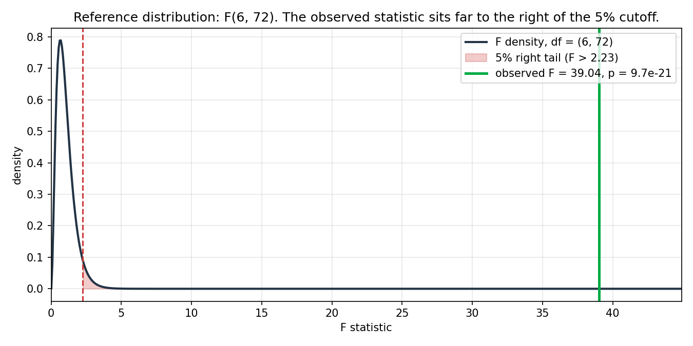
Three features matter for reading this picture.

1. The whole distribution lives at positive numbers, because F is a ratio of two non-negative variances. There is no left tail.
2. It is right-skewed and peaked just below 1. Under $H_0$, the most common value of F is right around 1 (the two MS quantities are both unbiased estimates of ${\sigma }^2$, so their ratio is on average 1). Ratios up to maybe 3 or 4 are not surprising even under $H_0$ — they just reflect the fact that a finite-sample variance estimate is itself noisy.
3. The right tail trails off fast. Past about $F=3$, the curve hugs the axis; past $F=5$, it is essentially invisible. The 5 % right-tail cutoff for $F(6,72)$, marked with the dashed red line, sits at $F^{\ast }=2.227$. Under $H_0$, only one F statistic in twenty exceeds this value.

The lack-of-fit test rejects $H_0$ if the observed F sits in this right tail — i.e., is bigger than $F^{\ast }$. The bigger the observed F, the smaller the right-tail area beyond it, and the smaller the p-value. For our data, the observed $F=39.04$ is so far to the right of the cutoff that it lies completely outside the visible part of the density curve, and the right-tail p-value is:

$$p=\mathrm{Pr}(F_{6,72}>39.04)\approx 9.7\times 10^{-21}.$$

For comparison, the $\alpha =0.001$ cutoff for $F(6,72)$ is about $4.26$, the $\alpha =0.0001$ cutoff is about $5.4$, and our observed $F$ is roughly seven times the latter. The chance of getting an F this large under the null hypothesis is essentially zero. We reject.

Connection to one-way ANOVA (for students whose teacher covered it)

If you have seen one-way ANOVA in AP Statistics, the construction here is structurally identical. In ANOVA, the F statistic is

$$F_{\text{ANOVA}}=\frac{{\mathrm{MS}}_{\text{between}}}{{\mathrm{MS}}_{\text{within}}},$$

asking whether the variability between group means is bigger than the variability within groups. Big F means the groups have different population means. The denominator is built from the same within-group residuals as our ${\mathrm{MS}}_{\text{PE}}$; the numerator measures how far the group means scatter from the overall mean. The lack-of-fit test reuses the within-group denominator unchanged and swaps the numerator to ask a different question: are the group means scattered around the line by more than within-group noise predicts? Same machinery, applied to a regression instead of a group-comparison.

Conditions for the test

The lack-of-fit F-test inherits LINER from the regression machinery, but with two important differences from the slope t-test:

1. L is the null hypothesis, not a pre-condition. Where the slope t-test needs to assume linearity before producing a trustworthy p-value, the lack-of-fit test is built precisely to test it. There is no L to check before running.
2. A new condition replaces L: $X$ must have repeated values. ${\mathrm{MS}}_{\text{PE}}$ is computed from within-bin spread; if every $X$ value occurs only once, the within-bin SS is zero, ${\mathrm{df}}_{\text{PE}}=n-k=0$, and the test is undefined. For the spring data, every mass has 10 replicates, so ${\mathrm{df}}_{\text{PE}}=72$, comfortably positive.

The remaining conditions are the familiar I, N, E, R — all checked and passing on the linear fit above. The lack-of-fit test on this dataset is therefore good to run.

Plugging the numbers in

The arithmetic uses two ingredients: ${\mathrm{SSE}}_{\text{lin}}$, which is in hand from the slope test, and ${\mathrm{SS}}_{\text{PE}}$, which is the sum of the within-bin sums of squared deviations. The latter is easiest to compute one bin at a time.

Per-bin within-SS

For each mass level $k$, the within-bin SS is ${\sum }_{i\in \text{bin }k}(y_i-{\bar{y}}_k{)}^2=(n_k-1)\cdot s_k^2$, where $s_k$ is the within-level SD already tabulated in the data tour. The eight values:

mass (g)	$n_k$	${\bar{y}}_k$	$s_k$	$\sum (y_i-{\bar{y}}_k{)}^2$
100	10	0.5817	0.1291	0.1500
200	10	1.1465	0.1499	0.2022
300	10	1.7894	0.1449	0.1891
400	10	2.8451	0.2533	0.5775
500	10	3.8083	0.1879	0.3179
600	10	4.8502	0.1311	0.1547
700	10	6.0678	0.1711	0.2636
800	10	7.4499	0.1258	0.1425

(The rightmost column is $9\cdot s_k^2$ for each row.) Summing the column gives the pure-error sum of squares:

$${\mathrm{SS}}_{\text{PE}}=0.1500+0.2022+0.1891+0.5775+0.3179+0.1547+0.2636+0.1425=\mathrm{1.9975.}$$

This is the irreducible noise — the part no smooth curve through eight $X$-levels could ever explain. Its degree of freedom: ${\mathrm{df}}_{\text{PE}}=n-k=80-8=72$.

Lack-of-fit sum of squares

The complement is the structured part the line failed to capture:

$${\mathrm{SS}}_{\text{LoF}}={\mathrm{SSE}}_{\text{lin}}-{\mathrm{SS}}_{\text{PE}}=8.4962-1.9975=6.4987,$$

with ${\mathrm{df}}_{\text{LoF}}=(n-2)-(n-k)=k-2=6$. As a sanity check, ${\mathrm{SS}}_{\text{LoF}}$ can also be computed directly as ${\sum }_k{n}_k({\bar{y}}_k-{\hat{y}}_k^{(\text{lin})}{)}^2$ using the per-bin "smile" deviations from the residual plot:

mass (g)	${\bar{y}}_k$	${\hat{y}}_k^{(\text{lin})}$	${\bar{y}}_k-{\hat{y}}_k^{(\text{lin})}$
100	0.5817	0.1161	$+0.4655$
200	1.1465	1.1022	$+0.0443$
300	1.7894	2.0882	$-0.2989$
400	2.8451	3.0743	$-0.2292$
500	3.8083	4.0604	$-0.2520$
600	4.8502	5.0464	$-0.1963$
700	6.0678	6.0325	$+0.0352$
800	7.4499	7.0186	$+0.4313$

(The line passes through the centroid $(\bar{x},\bar{y})=(450,3.567)$ with slope $0.009861$; ${\hat{y}}_k^{(\text{lin})}=\bar{y}+{\hat{\beta }}_1(x_k-\bar{x})$.) Multiplying each squared gap by $n_k=10$ and summing yields the same ${\mathrm{SS}}_{\text{LoF}}\approx 6.499$ — the two arithmetic paths agree, as the identity guarantees.

Mean squares and the F ratio

The two mean squares:

$${\mathrm{MS}}_{\text{LoF}}=\frac{6.4987}{6}=1.0831,{\mathrm{MS}}_{\text{PE}}=\frac{1.9975}{72}=\mathrm{0.02774.}$$

The F statistic:

$$F=\frac{{\mathrm{MS}}_{\text{LoF}}}{{\mathrm{MS}}_{\text{PE}}}=\frac{1.0831}{0.02774}=\mathrm{39.04.}$$

Reference distribution: $F(6,72)$, as set up in Step 7 above. The $\alpha =0.05$ critical value is $F^{\ast }(6,72)\approx 2.227$; the observed statistic is more than seventeen times larger. The right-tail p-value:

$$p=\mathrm{Pr}(F_{6,72}>39.04)\approx 9.7\times 10^{-21}.$$

Reading the result

Two p-values now describe the same dataset:

• Slope t-test: $t=61.23$, $p\approx 10^{-67}$. Reject $H_0:{\beta }_1=0$.
• Lack-of-fit F-test: $F=39.04$, $p\approx 10^{-21}$. Reject $H_0:\text{linear shape}$.

Both p-values are decisive, but they answer different questions and the conjunction matters. The honest one-sentence summary of the analysis is:

There is overwhelming evidence (i) that extension grows with mass, and (ii) that the growth is not linear.

The slope test alone gets you (i). It is the lack-of-fit test that gets you (ii), and the AP curriculum produces students who would have stopped at (i), reported "linear relationship", and missed a real piece of the physics.

What is the line missing? The pattern of bin residuals reveals the shape. The gap is positive at the small end ($+0.47$ at 100 g), negative through the middle, then positive again at the large end ($+0.43$ at 800 g) — a U-shape on the residual plot, which means a concave-up departure from the line. The natural follow-up is to fit a quadratic, $\hat{y}={\beta }_0+{\beta }_{1}x+{\beta }_2{x}^2$, which would absorb the curvature and bring the lack-of-fit statistic back toward 1. Whether the curvature is physically meaningful (the spring is being stretched past its proportional limit; Hooke's law is leaving the elastic regime) is a substantive physics question that the F-test does not answer — it only tells the analyst that the linear summary is leaving a real signal on the table.

There is one comforting piece of news. The slope estimate ${\hat{\beta }}_1=0.00986$ cm/g is not "wrong" in any deep sense; it is the best linear summary of a curved relationship, and the 95 % CI on it is honest under the LINER conditions that pass. What the lack-of-fit test forbids is the interpretation "extension is linear in mass" — that claim is the one the data rule out.

When you cannot run this test

The lack-of-fit F-test needs replicate $X$ values to function. The pure-error mean square is constructed from the within-bin spread, and if every $X$ value is observed exactly once, every "bin" has $n_k=1$ and contributes zero to the within-bin SS. The numerator and denominator of $F$ both collapse — ${\mathrm{df}}_{\text{PE}}=n-k=n-n=0$ — and the test is undefined.

Two practical responses are available when no replicates exist:

1. Cluster the $X$ values into near-replicates. If $X$ varies continuously but the experimenter designed the levels close enough together that "near-equal" $X$ is meaningful, the data can be grouped into bins and the lack-of-fit test run within each grouping. The cost is that "pure error" now includes a small amount of structural variation from the bin range, so the test is mildly anti-conservative. AP-level treatments do not cover this generalisation.
2. Switch diagnostics. Without replicates, the qualitative residual-plot inspection remains available, and so do model-comparison F-tests against a named alternative ("does adding $X^2$ improve the fit beyond what 1 extra parameter random would?"). Those are slope tests on the quadratic coefficient, not the omnibus lack-of-fit test, and they detect only the specific alternative they are designed for.

The spring experiment was designed with 10 replicates per level precisely so the lack-of-fit test would be available. Designing replicate structure into an experiment is one of the most important things an experimenter can do to keep diagnostic options open.

Connection back to AP Statistics

The whole construction uses nothing outside the AP curriculum. The ingredients are:

• Regression machinery: $\mathrm{SSE}$, ${\hat{\beta }}_0$, ${\hat{\beta }}_1$, residuals — covered in Unit 2 (one-variable regression) and Unit 9 (inference for regression).
• ANOVA / F-distribution: the F statistic as a ratio of mean squares, the right-tail rejection rule — covered in Unit 7 (inference for means) for one-way ANOVA, with the F-distribution and df bookkeeping appearing identically.
• Sum-of-squares decomposition: explicitly taught in the ANOVA section as ${\mathrm{SS}}_{\text{total}}={\mathrm{SS}}_{\text{between}}+{\mathrm{SS}}_{\text{within}}$. The lack-of-fit decomposition ${\mathrm{SSE}}_{\text{lin}}={\mathrm{SS}}_{\text{LoF}}+{\mathrm{SS}}_{\text{PE}}$ is the same identity in a different costume — between-bin vs. within-bin variation, viewed through the lens of "how much of the between-bin variation can a line explain?".

The only thing the AP curriculum does not do is combine these ingredients into the single nested-model F that tests a regression's L condition. That step is one course-worth of material past where AP stops, and yet it requires no new mathematical concept — only the willingness to apply ANOVA bookkeeping to the residuals of a regression. A student who has finished AP Stats has every tool needed to read this post, to run the same test on a different dataset, and to understand why "the slope is significant" is not the same statement as "the line is the right shape".

The lack-of-fit F-test made one related appearance earlier on this site, as Test C in the pot-vs-seats analysis, where it diagnosed a curve in 1238 poker hands on a log scale. The synthetic spring example here is the stripped-down version of the same machinery, designed so the only complication is the test itself rather than the dataset around it.

Materials

Everything used to produce this post is hosted alongside it.

• Main pipeline — lack-of-fit.py (14 KB). Generates the synthetic dataset with a fixed seed (np.random.default_rng(20260528)), runs the linear OLS slope test and the lack-of-fit F-test (both by hand and via statsmodels.stats.anova_lm), and writes every figure used in the post.
• Arithmetic walkthrough — lack-of-fit-arith.py (7 KB). Prints every intermediate sum ($\sum x$, $\sum y$, $S_{xx}$, $S_{yy}$, $S_{xy}$, ${\hat{\beta }}_1$, $\mathrm{SSE}$, per-bin within-SS, ${\mathrm{SS}}_{\text{LoF}}$, ${\mathrm{MS}}_{\text{LoF}}$, ${\mathrm{MS}}_{\text{PE}}$, $F$, $F^{\ast }$, $p$) so every by-hand quantity quoted in the post can be verified.

Both scripts depend on pandas, numpy, scipy, statsmodels, and matplotlib. Quickstart:

python3 -m venv .venv && source .venv/bin/activate
pip install pandas numpy scipy statsmodels matplotlib

python3 lack-of-fit.py         # full pipeline (figures + summary)
python3 lack-of-fit-arith.py   # detailed arithmetic

The whole computation runs in a couple of seconds on a modern laptop. For convenience, both scripts are included verbatim below.

lack-of-fit.py

#!/usr/bin/env python3
"""
Lack-of-fit F-test introduction — full pipeline.

Companion script to the blog post
"Beyond 'is the slope significant?': An introduction to the lack-of-fit F-test"

    https://www.sinostatistica.net/blog/lack-of-fit-intro

Walks through the lack-of-fit F-test on a synthetic spring-extension
dataset: 8 distinct mass levels (100, 200, ..., 800 g), 10 replicate
measurements at each level. The "truth" used to generate the data has
a small quadratic curvature on top of an otherwise linear extension,
so the linear regression slope is highly significant but the linear
shape is itself wrong.

Outputs:
    fig-data-scatter.png       raw data + bin means + would-be OLS line
    fig-residual-plot.png      residuals vs fitted (concave pattern)
    fig-nested-models.png      linear fit vs saturated (per-bin means)
    fig-ss-decomposition.png   SSE_lin = SS_PE + SS_LoF stacked bar
    fig-f-distribution.png     F(6, 72) density with stat + critical value

Run:      python3 lack-of-fit.py
Depends:  pandas, numpy, scipy, statsmodels, matplotlib.
"""
from __future__ import annotations

from pathlib import Path

import matplotlib.pyplot as plt
import numpy as np
import pandas as pd
import statsmodels.api as sm
import statsmodels.formula.api as smf
from scipy.stats import f as f_dist
from scipy.stats import t as student_t

# ---------------------------------------------------------------------------
# Configuration
# ---------------------------------------------------------------------------

HERE = Path(__file__).parent
OUT = HERE
RNG = np.random.default_rng(20260528)

MASS_LEVELS_G = np.array([100, 200, 300, 400, 500, 600, 700, 800])
REPLICATES = 10

# True data-generating process, kept in code only (never quoted as
# "the truth" in the blog post — the student sees the data as if it
# came out of a lab):
#
#     extension_cm = 0.45*(m/100) + 0.06*(m/100)^2 + N(0, 0.18^2)
#
# At m = 100 g this is 0.45 + 0.06 = 0.51 cm.
# At m = 800 g this is 3.60 + 3.84 = 7.44 cm.
TRUE_BETA_LIN = 0.45     # cm per (100 g)
TRUE_BETA_QUAD = 0.06    # cm per (100 g)^2
NOISE_SD = 0.18          # cm


# ---------------------------------------------------------------------------
# Data
# ---------------------------------------------------------------------------

def make_dataset() -> pd.DataFrame:
    """Generate the synthetic spring-extension dataset."""
    masses = np.repeat(MASS_LEVELS_G, REPLICATES).astype(float)
    m100 = masses / 100.0
    truth = TRUE_BETA_LIN * m100 + TRUE_BETA_QUAD * m100 ** 2
    noise = RNG.normal(0.0, NOISE_SD, size=len(masses))
    extensions = truth + noise
    return pd.DataFrame({"mass_g": masses, "extension_cm": extensions})


# ---------------------------------------------------------------------------
# Test machinery
# ---------------------------------------------------------------------------

def linear_fit(df: pd.DataFrame):
    return smf.ols("extension_cm ~ mass_g", data=df).fit()


def lack_of_fit_table(df: pd.DataFrame, lin_fit):
    sat_fit = smf.ols("extension_cm ~ C(mass_g)", data=df).fit()
    return sm.stats.anova_lm(lin_fit, sat_fit), sat_fit


def summarise(df: pd.DataFrame) -> None:
    n = len(df)
    print(f"n observations             : {n}")
    print(f"distinct mass levels (k)   : {df.mass_g.nunique()}")
    bin_summary = (df.groupby("mass_g")
                     .agg(n=("extension_cm", "size"),
                          mean=("extension_cm", "mean"),
                          sd=("extension_cm", "std"))
                     .round(4))
    print("\n=== Per-mass-level summary ===")
    print(bin_summary.to_string())

    lin = linear_fit(df)
    print("\n=== Linear OLS fit ===")
    print(f"  beta_0 = {lin.params['Intercept']:.6f} cm")
    print(f"  beta_1 = {lin.params['mass_g']:.6f} cm/g")
    print(f"  SE(beta_1) = {lin.bse['mass_g']:.6f}")
    print(f"  t = {lin.tvalues['mass_g']:.4f}")
    print(f"  p = {lin.pvalues['mass_g']:.3g}")
    print(f"  R^2 = {lin.rsquared:.4f}")
    print(f"  SSE_lin = {lin.ssr:.4f},  df_lin = {int(lin.df_resid)}")
    tstar = student_t.ppf(0.975, lin.df_resid)
    ci_lo, ci_hi = lin.conf_int().loc["mass_g"]
    print(f"  t*(0.975, {int(lin.df_resid)}) = {tstar:.4f}")
    print(f"  95% CI on beta_1 = [{ci_lo:.6f}, {ci_hi:.6f}] cm/g")

    anova, sat = lack_of_fit_table(df, lin)
    print("\n=== Saturated OLS fit (one mean per mass level) ===")
    print(f"  SS_PE = {sat.ssr:.4f},  df_PE = {int(sat.df_resid)}")

    SSE_lin = lin.ssr
    SS_PE = sat.ssr
    df_lin = int(lin.df_resid)
    df_PE = int(sat.df_resid)
    SS_LoF = SSE_lin - SS_PE
    df_LoF = df_lin - df_PE
    MS_LoF = SS_LoF / df_LoF
    MS_PE = SS_PE / df_PE
    F = MS_LoF / MS_PE
    p_F = f_dist.sf(F, df_LoF, df_PE)
    Fcrit = f_dist.ppf(0.95, df_LoF, df_PE)

    print("\n=== Lack-of-fit F-test ===")
    print(f"  SS_LoF = {SS_LoF:.4f},  df_LoF = {df_LoF}")
    print(f"  MS_LoF = {MS_LoF:.4f},  MS_PE = {MS_PE:.4f}")
    print(f"  F      = {F:.4f}")
    print(f"  F*(0.05, {df_LoF}, {df_PE}) = {Fcrit:.4f}")
    print(f"  p(F_{df_LoF},{df_PE} > {F:.2f}) = {p_F:.3g}")


# ---------------------------------------------------------------------------
# Figures (see online file for full implementation)
# ---------------------------------------------------------------------------

def fig_data_scatter(df, lin):
    xs = np.linspace(MASS_LEVELS_G.min() - 20, MASS_LEVELS_G.max() + 20, 100)
    fitted = lin.params["Intercept"] + lin.params["mass_g"] * xs
    bin_mean = df.groupby("mass_g").extension_cm.mean()
    fig, ax = plt.subplots(figsize=(9, 5))
    jitter = RNG.uniform(-8, 8, len(df))
    ax.scatter(df.mass_g + jitter, df.extension_cm,
               s=24, alpha=0.45, color="#444", linewidth=0,
               label=f"raw measurements (n = {len(df)})")
    ax.scatter(bin_mean.index, bin_mean.values,
               s=120, color="#0a4", zorder=5, edgecolor="white",
               linewidth=1.8, label="per-mass mean extension")
    ax.plot(xs, fitted, color="#c33", linewidth=2.2,
            label=f"linear OLS fit: extension = "
                  f"{lin.params['Intercept']:.3f} + "
                  f"{lin.params['mass_g']:.5f} . mass")
    ax.set_xlabel("Mass on the spring (g)")
    ax.set_ylabel("Extension below the rest length (cm)")
    ax.set_xticks(MASS_LEVELS_G)
    ax.grid(alpha=0.3)
    ax.legend(loc="upper left")
    fig.tight_layout()
    fig.savefig(OUT / "fig-data-scatter.png", dpi=150)
    plt.close(fig)


def fig_residual_plot(df, lin):
    fitted = lin.fittedvalues.to_numpy()
    resid = lin.resid.to_numpy()
    bin_mean_resid = (pd.DataFrame({"mass_g": df.mass_g, "resid": resid})
                        .groupby("mass_g").resid.mean())
    bin_fitted = (lin.params["Intercept"]
                  + lin.params["mass_g"] * bin_mean_resid.index.to_numpy())
    fig, ax = plt.subplots(figsize=(9, 4.7))
    ax.axhline(0, color="black", linewidth=0.8)
    ax.scatter(fitted, resid, s=24, alpha=0.45, color="#444", linewidth=0)
    ax.plot(bin_fitted, bin_mean_resid.values, "o-",
            color="#c33", markersize=9, linewidth=2,
            label="mean residual at each mass level")
    ax.set_xlabel("Fitted value (cm)")
    ax.set_ylabel("Residual (cm)")
    ax.grid(alpha=0.3)
    ax.legend(loc="upper left")
    fig.tight_layout()
    fig.savefig(OUT / "fig-residual-plot.png", dpi=150)
    plt.close(fig)


def fig_nested_models(df, lin):
    bin_mean = df.groupby("mass_g").extension_cm.mean()
    bin_sd = df.groupby("mass_g").extension_cm.std()
    bin_n = df.groupby("mass_g").extension_cm.size()
    bin_se = bin_sd / np.sqrt(bin_n)
    xs = np.linspace(MASS_LEVELS_G.min() - 20, MASS_LEVELS_G.max() + 20, 100)
    fitted = lin.params["Intercept"] + lin.params["mass_g"] * xs
    fig, (axL, axR) = plt.subplots(1, 2, figsize=(13, 5), sharey=True)
    jitter = RNG.uniform(-8, 8, len(df))
    axL.scatter(df.mass_g + jitter, df.extension_cm, s=20,
                alpha=0.30, color="#666", linewidth=0)
    axL.plot(xs, fitted, color="#c33", linewidth=2.2,
             label="linear model (2 parameters)")
    axL.set_title("Linear model")
    axR.scatter(df.mass_g + jitter, df.extension_cm, s=20,
                alpha=0.30, color="#666", linewidth=0)
    axR.errorbar(bin_mean.index, bin_mean.values,
                 yerr=1.96 * bin_se, fmt="o-",
                 color="#06a", markersize=9, linewidth=2, capsize=4,
                 label="saturated model (8 parameters)")
    axR.set_title("Saturated model")
    for ax in (axL, axR):
        ax.set_xlabel("Mass (g)")
        ax.set_xticks(MASS_LEVELS_G)
        ax.grid(alpha=0.3)
        ax.legend(loc="upper left")
    axL.set_ylabel("Extension (cm)")
    fig.tight_layout()
    fig.savefig(OUT / "fig-nested-models.png", dpi=150)
    plt.close(fig)


def fig_ss_decomposition(SSE_lin, SS_PE, SS_LoF):
    fig, ax = plt.subplots(figsize=(7, 5))
    ax.bar(0, SS_PE, width=0.55, color="#06a",
           label=f"pure error: SS_PE = {SS_PE:.4f}")
    ax.bar(0, SS_LoF, bottom=SS_PE, width=0.55, color="#c33",
           label=f"lack of fit: SS_LoF = {SS_LoF:.4f}")
    ax.set_xticks([0])
    ax.set_xticklabels([f"SSE_lin = {SSE_lin:.4f}"])
    ax.set_ylabel("Sum of squared residuals (cm$^2$)")
    ax.legend(loc="upper right")
    fig.tight_layout()
    fig.savefig(OUT / "fig-ss-decomposition.png", dpi=150)
    plt.close(fig)


def fig_f_distribution(F_obs, df_LoF, df_PE):
    Fcrit = f_dist.ppf(0.95, df_LoF, df_PE)
    p = f_dist.sf(F_obs, df_LoF, df_PE)
    xmax = max(F_obs * 1.15, Fcrit * 2.0, 6.0)
    xs = np.linspace(0.01, xmax, 600)
    ys = f_dist.pdf(xs, df_LoF, df_PE)
    fig, ax = plt.subplots(figsize=(9, 4.5))
    ax.plot(xs, ys, color="#234", linewidth=2,
            label=f"F density, df = ({df_LoF}, {df_PE})")
    tail_xs = xs[xs >= Fcrit]
    tail_ys = ys[xs >= Fcrit]
    ax.fill_between(tail_xs, 0, tail_ys, color="#c33", alpha=0.25,
                    label=f"5% right tail (F > {Fcrit:.2f})")
    ax.axvline(Fcrit, color="#c33", linestyle="--", linewidth=1.4)
    ax.axvline(F_obs, color="#0a4", linewidth=2.4,
               label=f"observed F = {F_obs:.2f}, p = {p:.2g}")
    ax.set_xlabel("F statistic")
    ax.set_ylabel("density")
    ax.set_xlim(0, xmax)
    ax.grid(alpha=0.3)
    ax.legend(loc="upper right")
    fig.tight_layout()
    fig.savefig(OUT / "fig-f-distribution.png", dpi=150)
    plt.close(fig)


# ---------------------------------------------------------------------------
# Main
# ---------------------------------------------------------------------------

def main():
    df = make_dataset()
    lin = linear_fit(df)
    _, sat = lack_of_fit_table(df, lin)
    summarise(df)
    SSE_lin = lin.ssr
    SS_PE = sat.ssr
    SS_LoF = SSE_lin - SS_PE
    df_LoF = int(lin.df_resid - sat.df_resid)
    df_PE = int(sat.df_resid)
    F_obs = (SS_LoF / df_LoF) / (SS_PE / df_PE)
    fig_data_scatter(df, lin)
    fig_residual_plot(df, lin)
    fig_nested_models(df, lin)
    fig_ss_decomposition(SSE_lin, SS_PE, SS_LoF)
    fig_f_distribution(F_obs, df_LoF, df_PE)
    print("\nAll figures written to:", OUT)


if __name__ == "__main__":
    main()

lack-of-fit-arith.py

#!/usr/bin/env python3
"""
Lack-of-fit F-test introduction — arithmetic walkthrough.

Companion to lack-of-fit.py. Prints every intermediate quantity that
the blog post plugs into a formula by hand: X- and Y-sums, beta_0,
beta_1, SSE, R^2, s, SE, t, p, t*, 95% CI, per-bin within-SS, SS_PE,
SS_LoF, MS_LoF, MS_PE, F, F*(0.05), p_F.

Run:      python3 lack-of-fit-arith.py
Depends:  numpy, pandas, scipy.
"""
from __future__ import annotations

import numpy as np
import pandas as pd
from scipy.stats import f as f_dist
from scipy.stats import t as student_t

RNG = np.random.default_rng(20260528)
MASS_LEVELS_G = np.array([100, 200, 300, 400, 500, 600, 700, 800])
REPLICATES = 10
TRUE_BETA_LIN = 0.45
TRUE_BETA_QUAD = 0.06
NOISE_SD = 0.18

masses = np.repeat(MASS_LEVELS_G, REPLICATES).astype(float)
m100 = masses / 100.0
truth = TRUE_BETA_LIN * m100 + TRUE_BETA_QUAD * m100 ** 2
noise = RNG.normal(0.0, NOISE_SD, size=len(masses))
extensions = truth + noise

x = masses
y = extensions
n = len(x)
k = len(np.unique(x))

xbar = x.mean()
ybar = y.mean()
Sxx = ((x - xbar) ** 2).sum()
Syy = ((y - ybar) ** 2).sum()
Sxy = ((x - xbar) * (y - ybar)).sum()

beta1 = Sxy / Sxx
beta0 = ybar - beta1 * xbar
yhat = beta0 + beta1 * x
SSE_lin = ((y - yhat) ** 2).sum()
R2 = 1 - SSE_lin / Syy
df_lin_resid = n - 2
s = np.sqrt(SSE_lin / df_lin_resid)
SE_b1 = s / np.sqrt(Sxx)
t_stat = beta1 / SE_b1
p_t = 2 * student_t.sf(abs(t_stat), df_lin_resid)
tstar = student_t.ppf(0.975, df_lin_resid)
ci = (beta1 - tstar * SE_b1, beta1 + tstar * SE_b1)

print("=== Linear OLS arithmetic ===")
print(f"n                = {n}")
print(f"k (mass levels)  = {k}")
print(f"xbar             = {xbar:.6f}")
print(f"ybar             = {ybar:.6f}")
print(f"Sxx              = {Sxx:.4f}")
print(f"Syy = SST        = {Syy:.6f}")
print(f"Sxy              = {Sxy:.4f}")
print(f"beta_1_hat       = {beta1:.8f}")
print(f"beta_0_hat       = {beta0:.6f}")
print(f"SSE_lin          = {SSE_lin:.6f}")
print(f"R^2              = {R2:.6f}")
print(f"s                = {s:.6f}")
print(f"SE(beta_1)       = {SE_b1:.8f}")
print(f"t                = {t_stat:.4f}")
print(f"two-sided p      = {p_t:.4g}")
print(f"t*(0.975, {df_lin_resid})   = {tstar:.4f}")
print(f"95% CI on beta_1 = [{ci[0]:.6f}, {ci[1]:.6f}] cm/g\n")

df = pd.DataFrame({"mass_g": x, "extension_cm": y})
bin_stats = (df.groupby("mass_g")
               .agg(n_k=("extension_cm", "size"),
                    mean_y=("extension_cm", "mean"),
                    sumsq_dev=("extension_cm",
                               lambda v: ((v - v.mean()) ** 2).sum()))
               .reset_index())

print("=== Per-mass-level (saturated model) arithmetic ===")
print(f"{'mass_g':>8} {'n_k':>4} {'mean_y':>10} {'sumsq_dev':>14}")
for _, row in bin_stats.iterrows():
    print(f"{int(row.mass_g):>8} {int(row.n_k):>4} "
          f"{row.mean_y:>10.4f} {row.sumsq_dev:>14.6f}")

SS_PE = bin_stats.sumsq_dev.sum()
df_PE = n - k
print(f"\nSS_PE = {SS_PE:.6f},  df_PE = {df_PE}\n")

SS_LoF = SSE_lin - SS_PE
df_LoF = df_lin_resid - df_PE
MS_LoF = SS_LoF / df_LoF
MS_PE = SS_PE / df_PE
F = MS_LoF / MS_PE
p_F = f_dist.sf(F, df_LoF, df_PE)
Fcrit = f_dist.ppf(0.95, df_LoF, df_PE)

print("=== Lack-of-fit F-test arithmetic ===")
print(f"SS_LoF = SSE_lin - SS_PE   = {SS_LoF:.6f}")
print(f"df_LoF = k - 2             = {df_LoF}")
print(f"df_PE  = n - k             = {df_PE}")
print(f"MS_LoF = SS_LoF / df_LoF   = {MS_LoF:.6f}")
print(f"MS_PE  = SS_PE  / df_PE    = {MS_PE:.6f}")
print(f"F      = MS_LoF / MS_PE    = {F:.6f}")
print(f"F*(0.05, {df_LoF}, {df_PE})      = {Fcrit:.4f}")
print(f"p(F_{df_LoF},{df_PE} > {F:.4f}) = {p_F:.3g}")

bin_stats["lin_pred"] = beta0 + beta1 * bin_stats.mass_g
bin_stats["bin_resid"] = bin_stats.mean_y - bin_stats.lin_pred
print("\n=== Per-bin residual (mean_y - linear prediction) ===")
print(f"{'mass_g':>8} {'mean_y':>10} {'lin_pred':>10} {'resid':>10}")
for _, row in bin_stats.iterrows():
    print(f"{int(row.mass_g):>8} {row.mean_y:>10.4f} "
          f"{row.lin_pred:>10.4f} {row.bin_resid:>+10.4f}")